


As of August 2017, Twitter had 328 million active users, with 500 million tweets being sent every day. Let’s look at how the open source R programming language can be used to analyse the tremendous amount of data created by this very popular social media tool.
Social networking websites are ideal sources of Big Data, which has many applications in the real world. These sites contain both structured and unstructured data, and are perfect platforms for data mining and subsequent knowledge discovery from the source. Twitter is a popular source of text data for data mining. Huge volumes of Twitter data contain many varieties of topics, which can be analysed to study the trends of different current subjects, like market economics or a wide variety of social issues. Accessing Twitter data is easy as open APIs are available to transfer and arrange data in JSON and ATOM formats.
In this article, we will look at an R programming implementation for Twitter data analysis and visualisation. This will give readers an idea of how to use R to analyse Big Data. As a micro blogging network for the exchange and sharing of short public messages, Twitter provides a rich repository of different hyperlinks, multimedia and hashtags, depicting the contemporary social scenario in a geolocation. From the originating tweets and the responses to them, as well as the retweets by other users, it is possible to implement opinion mining over a subject of interest in a geopolitical location. By analysing the favourite counts and the information about the popularity of users in their followers’ count, it is also possible to make a weighted statistical analysis of the data.
Start your exploration
Exploring Twitter data using R requires some preparation. First, you need to have a Twitter account. Using that account, register an application into your Twitter account from https://apps.twitter.com/ site. The registration process requires basic personal information and produces four keys for R application and Twitter application connectivity. For example, an application myapptwitterR1 may be created as shown in Figure 1.
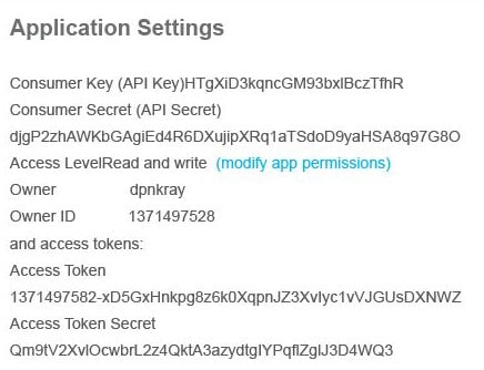
In turn, this will create your application settings, as shown in Figure 2.
A customer key, a customer secret, an access token and the access token secret combination forms the final authentication using the setup_twitter_oauth() function.
>setup_twitter_oauth(consumerKey, consumerSecret,AccessToken,AccessTokenSecret)
It is also necessary to create an object to save the authentication for future use. This is done by OAuthFactory$new() as follows:
credential<- OAuthFactory$new(consumerKey, consumerSecret, requestURL, accessURL,authURL)
Here, requestURL, accessURL and authURL are available from the application setting of https://apps.twitter.com/.
Connect to Twitter
This exercise requires R to have a few packages for calling all Twitter related functions. Here is an R script to start the Twitter data analysis task. To access the Twitter data through the just created application myapptwitterR, one needs to call twitter, ROAuth and modest packages.
>setwd(‘d:\\r\\twitter’)

>install.packages(“twitteR”)

>install.packages(“ROAuth”)

>install.packages(“modest”)

>library(“twitteR”)

>library(“ROAuth”)

>library(“httr”)
To test this on the MS Windows platform, load Curl into the current workspace, as follows:
>download.file (url=”http://curl.haxx.se/ca/cacert.pem”,destfile=”cacert.pem”)
Before the final connectivity to the Twitter application, save all the necessary key values to suitable variables:
>consumerKey=’HTgXiD3kqncGM93bxlBczTfhR’

>consumerSecret=’djgP2zhAWKbGAgiEd4R6DXujipXRq1aTSdoD9yaHSA8q97G8Oe’

>requestURL=’https://api.twitter.com/oauth/request_token’,

>accessURL=’https://api.twitter.com/oauth/access_token’,

>authURL=’https://api.twitter.com/oauth/authorize’)
With these preparations, one can now create the required connectivity object:
>cred<- OAuthFactory$new(consumerKey,consumerSecret,requestURL,accessURL,authURL)

>cred$handshake(cainfo=”cacert.pem”)
Authentication to a Twitter application is done by the function setup_twitter_oauth() with the stored key values as:
>setup_twitter_oauth(consumerKey, consumerSecret,AccessToken,AccessTokenSecret)
With all this done successfully, we are ready to access Twitter data. As an example of data analysis, let us consider the simple problem of opinion mining.
Data analysis
To demonstrate how data analysis is done, let’s get some data from Twitter. The Twitter package provides the function searchTwitter() to retrieve a tweet based on the keywords searched for. Twitter organises tweets using hashtags. With the help of a hashtag, you can expose your message to an audience interested in only some specific subject. If the hashtag is a popular keyword related to your business, it can act to increase your brand’s awareness levels. The use of popular hashtags helps one to get noticed. Analysis of hashtag appearances in tweets or Instagram can reveal different trends of what the people are thinking about the hashtag keyword. So this can be a good starting point to decide your business strategy.
To demonstrate hashtag analysis using R, here, we have picked up the number one hashtag keyword #love for the study. Other than this search keyword, the searchTwitter() function also requires the maximum number of tweets that the function call will return from the tweets. For this discussion, let us consider the maximum number as 500. Depending upon the speed of your Internet and the traffic on the Twitter server, you will get an R list class object responses within a few minutes and an R list class object.
>tweetList<- searchTwitter(“#love”,n=500)

>mode(tweetList)

[1] “list”

>length(tweetList)

[1] 500
In R, an object list is a compound data structure and contains all types of R objects, including itself. For further analysis, it is necessary to investigate its structure. Since it is an object of 500 list items, the structure of the first item is sufficient to understand the schema of the set of records.
>str(head(tweetList,1))

List of 1

$ :Reference class ‘status’ [package “twitteR”] with 20 fields

..$ text : chr “https://t.co/L8dGustBQX #SavOne #LLOVE #GotItWrong #JCole #Drake #Love #F4F #follow #follow4follow #Repost #followback”

..$ favorited : logi FALSE

..$ favoriteCount :num 0

..$ replyToSN : chr(0)

..$ created : POSIXct[1:1], format: “2017-10-04 06:11:03”

..$ truncated : logi FALSE

..$ replyToSID : chr(0)

..$ id : chr “915459228004892672”

..$ replyToUID : chr(0)

..$ statusSource :chr “<a href=\”http://twitter.com\” rel=\”nofollow\”>Twitter Web Client</a>”

..$ screenName : chr “Lezzardman”

..$ retweetCount : num 0

..$ isRetweet : logi FALSE

..$ retweeted : logi FALSE

..$ longitude : chr(0)

..$ latitude : chr(0)

..$ location :chr “Bay Area, CA, #CLGWORLDWIDE <ed><U+00A0><U+00BD><ed><U+00B2><U+00AF>”

..$ language : chr “en”

..$profileImageURL:chrhttp://pbs.twimg.com/profile_images/444325116407603200/XmZ92DvB_normal.jpeg”

..$ urls :’data.frame’: 1 obs. of 5 variables:

.. ..$ url : chr “https://t.co/L8dGustBQX”

.. ..$ expanded_url: chr “http://cdbaby.com/cd/savone”

.. ..$ display_url :chr “cdbaby.com/cd/savone”

.. ..$ start_index :num 0

.. ..$ stop_index :num 23

..and 59 methods, of which 45 are possibly relevant:

.. getCreated, getFavoriteCount, getFavorited, getId, getIsRetweet,

.. getLanguage, getLatitude, getLocation, getLongitude, getProfileImageURL,

.. getReplyToSID, getReplyToSN, getReplyToUID, getRetweetCount,

.. getRetweeted, getRetweeters, getRetweets, getScreenName, getStatusSource,

.. getText, getTruncated, getUrls, initialize, setCreated, setFavoriteCount,

.. setFavorited, setId, setIsRetweet, setLanguage, setLatitude, setLocation,

.. setLongitude, setProfileImageURL, setReplyToSID, setReplyToSN,

.. setReplyToUID, setRetweetCount, setRetweeted, setScreenName,

.. setStatusSource, setText, setTruncated, setUrls, toDataFrame,

.. toDataFrame#twitterObj

>
The structure shows that there are 20 fields of each list item, and the fields contain information and data related to the tweets.
Since the data frame is the most efficient structure for processing records, it is now necessary to convert each list item to the data frame and bind these row-by-row into a single frame. This can be done in an elegant way using the do.call() function call, as shown here:
loveDF<- do.call(“rbind”,lapply(tweetList, as.data.frame))
Function lapply() will first convert each list to a data frame, then do.call() will bind these, one by one. Now we have a set of records with 19 fields (one less than the list!) in a regular format ready for analysis. Here, we shall mainly consider ‘created’ field to study the distribution pattern of arrival of tweets.
>length(head(loveDF,1))

[1] 19

>str(head(lovetDF,1))

‘data.frame’ : 1 obs. of 19 variables:

$ text : chr “https://t.co/L8dGustBQX #SavOne #LLOVE #GotItWrong #JCole #Drake #Love #F4F #follow #follow4follow #Repost #followback”

$ favorited : logi FALSE

$ favoriteCount : num 0

$ replyToSN : chr NA

$ created : POSIXct, format: “2017-10-04 06:11:03”

$ truncated : logi FALSE

$ replyToSID : chr NA

$ id : chr “915459228004892672”

$ replyToUID : chr NA

$ statusSource : chr “<a href=\”http://twitter.com\” rel=\”nofollow\”>Twitter Web Client</a>”

$ screenName : chr “Lezzardman”

$ retweetCount : num 0

$ isRetweet : logi FALSE

$ retweeted : logi FALSE

$ longitude : chr NA

$ latitude : chr NA

$ location : chr “Bay Area, CA, #CLGWORLDWIDE <ed><U+00A0><U+00BD><ed><U+00B2><U+00AF>”

$ language : chr “en”

$ profileImageURL: chr “http://pbs.twimg.com/profile_images/444325116407603200/XmZ92DvB_normal.jpeg”

>
The fifth column field is ‘created’; we shall try to explore the different statistical characteristics features of this field.
>attach(loveDF) # attach the frame for further processing.

>head(loveDF[‘created’],2) # first 2 record set items for demo.

created

1 2017-10-04 06:11:03

2 2017-10-04 06:10:55
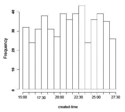
Twitter follows the Coordinated Universal Time tag as the time-stamp to record the tweet’s time of creation. This helps to maintain a normalised time frame for all records, and it becomes easy to draw a frequency histogram of the ‘created’ time tag.
>hist(created,breaks=15,freq=TRUE,main=”Histogram of created time tag”)
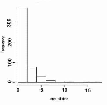
If we want to study the pattern of how the word ‘love’ appears in the data set, we can take the differences of consecutive time elements of the vector ‘created’. R function diff() can do this. It returns iterative lagged differences of the elements of an integer vector. In this case, we need lag and iteration variables as one. To have a time series from the ‘created’ vector, it first needs to be converted to an integer; here, we have done it before creating the series, as follows:
>detach(loveDF)

>sortloveDF<-loveDF[order(as.integer(created)),]

>attach(sortloveDF)

>hist(as.integer(abs(diff(created)))
This distribution shows that the majority of tweets in this group come within the first few seconds and a much smaller number of tweets arrive in subsequent time intervals. From the distribution, it’s apparent that the arrival time distribution follows a Poisson Distribution pattern, and it is now possible to model the number of times an event occurs in a given time interval.
Let’s check the cumulative distribution pattern, and the number of tweets arriving within a time interval. For this we have to write a short R function to get the cumulative values within each interval. Here is the demo script and the graph plot:
countarrival<- function(created)

{

i=1

s <- seq(1,15,1)

for(t in seq(1,15,1))

{

s[i] <- sum((as.integer(abs(diff(created))))<t)/500

i=i+1

}

return(s)

}
To create a cumulative value of the arriving tweets within a given interval, countarrival() uses sum() function over diff() function after converting the values into an integer.
>s <-countarrival(created)

>x<-seq(1,15,1)

>y<-s

>lo<- loess(y~x)

>plot(x,y)

>lines(predict(lo), col=’red’, lwd=2)

# sum((as.integer(abs(diff(created))))<t)/500
To have a smooth time series curve, the loess() function has been used with the predict() function. Predicted values based on the linear regression model, as provided by loess(), are plotted along with the x-y frequency values.
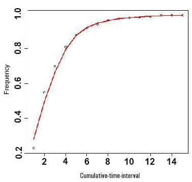
This is a classic example of probability distribution of arrival probabilities. The pattern in Figure 5 shows a cumulative Poisson Distribution, and can be used to model the number of events occurring within a given time interval. The X-axis contains one-second time intervals. Since this is a cumulative probability plot, the likelihood of the next tweet arriving corresponds to the X-axis value or less than that. For instance, since 4 on the X-axis approximately corresponds to 60 per cent on the Y-axis, the next tweet will arrive in 4 seconds or less than that time interval. In conclusion, we can say that all the events are mutually independent and occur at a known and constant rate per unit time interval.
This data analysis and visualisation shows that the arrival pattern is random and follows the Poisson Distribution. The reader may test the arrival pattern with a different keyword too.


