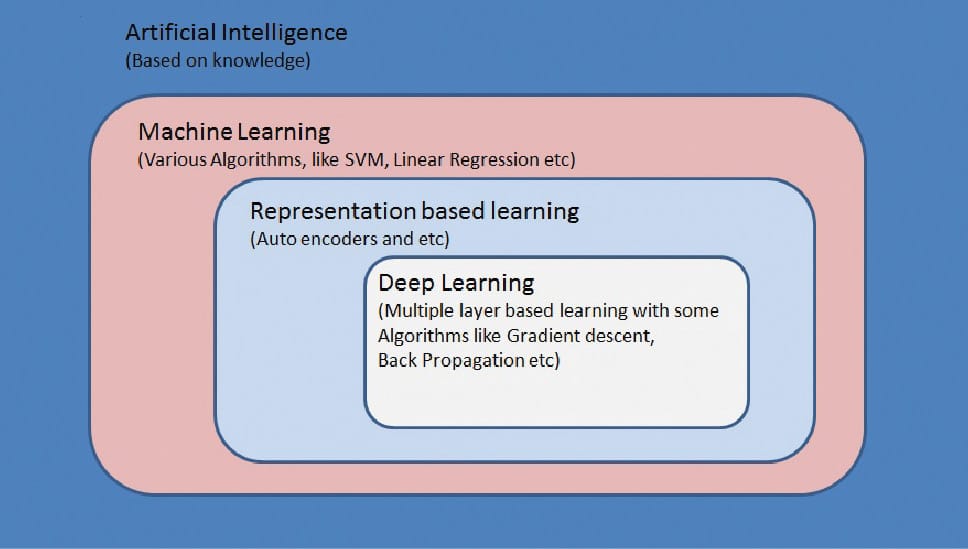
Deep Learning: Using Algorithms to Make Machines Think

Deep learning is part of the broader family of machine learning methods. It was introduced with the objective of moving machine learning closer to its main goal—that of artificial intelligence.

The human brain has evolved over many, many years and is one of our most important organs. The brain perceives every smell, taste, touch, sound and sight. Many decisions are taken by the brain every nano second, without our knowledge.

Having evolved over several thousands of years, the human brain has become a very sophisticated, complex and intelligent machine. What was not possible even as a dream during the 18th century and the beginning of the 19th century has become child’s play now in terms of technology. Many adult brains can recognise multiple complex situations and take decisions very, very fast because of this evolution. The brain learns new things very fast now and takes decisions quickly, compared to those taken a few decades ago.

A human now has access to vast amounts of information and processes a huge amount of data, day after day, and is able to digest all of it very quickly.

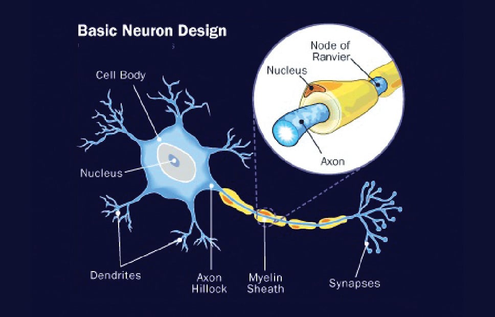
Our brain is made up of approximately 100 billion nerve cells, called neurons, which have the amazing ability to gather and transmit electrochemical signals. We can think of them as the gates and wires in a computer. Each of our experiences, senses and various normal functions trigger a lot of neuron based reactions/communications. Figure 1 shows the parts of a basic neuron.

The human brain and its neural network have been the subject of extensive research for the last several years, leading to the development of AI and machine learning technologies. The decade-long dream of building intelligent machines with brains like ours has finally materialised. Many complex problems can be now solved using deep learning techniques and algorithms. The simulation of human brain-like activities is becoming more plausible every moment.

How different is deep learning compared to machine learning

Machine learning was defined by Arthur Samuel as, “The field of study that gives computers the ability to learn without being explicitly programmed.” This was back in 1959.

In machine learning, computers are taught to solve certain problems with massive lists of rules, and are provided with models. In deep learning, the model provided can be evaluated with examples and a small set of instructions to modify it when it makes a mistake. Over time, a suitable model is able to solve the problem extremely accurately. That is why deep learning has become very popular and is catching every one’s eye. In the book ‘Fundamentals of Deep Learning’, the authors Nikhil Buduma and Nicholas Locascio state: “Deep learning is a subset of a more general field of artificial intelligence called machine learning, which is predicated on this idea of learning from example.”

Deep learning explained in detail

According to the free tutorial website computer4everyone.com, “Deep learning is a sub-field of machine learning concerned with algorithms inspired by the structure and function of the brain called artificial neural networks.”

Andrew Ng, who formally founded Google Brain, which eventually resulted in the commercialisation of deep learning technologies across a large number of Google services, has spoken and written a lot about deep learning. In his early talks on deep learning, Ng described deep learning in the context of traditional artificial neural networks.

At this point, it would be unfair if I did not mention other experts who have contributed to the field of deep learning. They include:

• Geoffrey Hinton for restricted Boltzmann machines stacked as deep-belief networks (sometimes he is referred to as the father of machine learning)
• Yann LeCun for convolutional networks (he was a student of Hinton)
• Yoshua Bengio, whose team has developed Theano (an open source solution for deep learning)
• Juergen Schmidhuber, who developed recurrent nets and LSTMs (long short-term memory, which is a recurrent neural network (RNN) architecture)

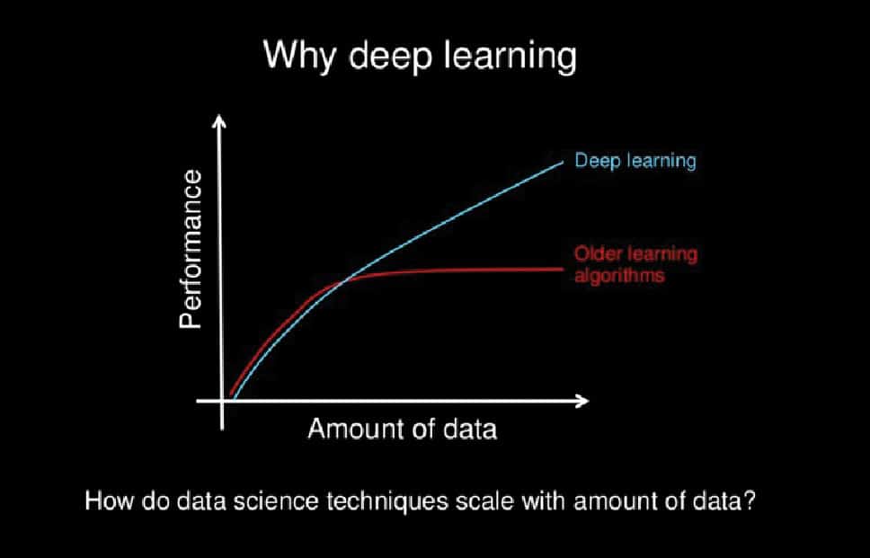
According to Andrew Ng, because of the huge volumes of data now available for computation and the recent advances in algorithms, deep learning technology has been adopted across the globe pretty quickly.

The potential for applications of deep learning in the modern world is humongous. Application fields include speech synthesis, learning based on past history, facial recognition, self-driving cars, medical sciences, stock predictions, and real estate rate predictions, to name a few.

Prerequisites to understanding deep learning technologies

There are a number of discussion forums and blogs on whether one has to know deep mathematics to understand deep learning. In my view, this should be evaluated on a case-to-case basis. Having said that, it is better to know the following if you really want to understand deep learning and are serious about it:

• The basic functions of neural networks
• An understanding of the basics of calculus
• An understanding of matrices, vectors and linear algebra
• Algorithms (supervised, unsupervised, online, batch, etc)
• Python programming
• Case-to-case basis mathematical equations

Note 1: In this article, I have tried my best to make you understand the basic concepts of deep learning, the differences between machine learning and AI, as well as some basic algorithms. The scope of this article does not allow a description of all the algorithms with mathematical functions.

Basics about neural networks

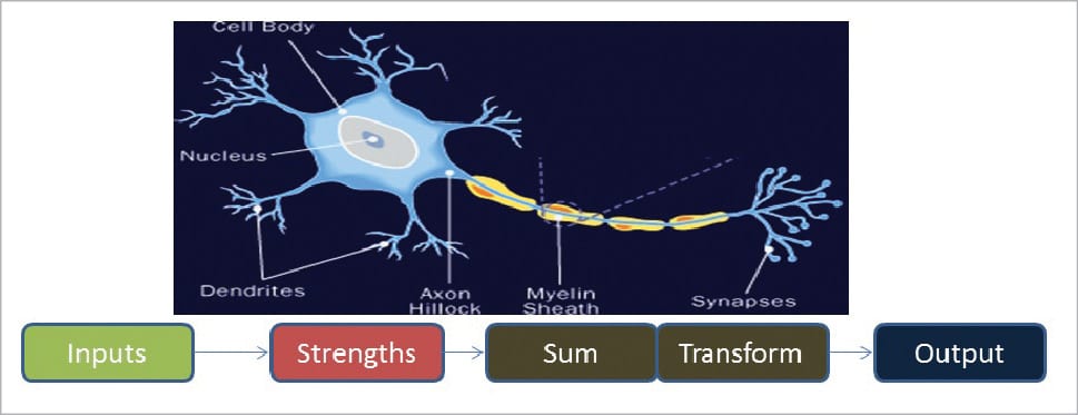
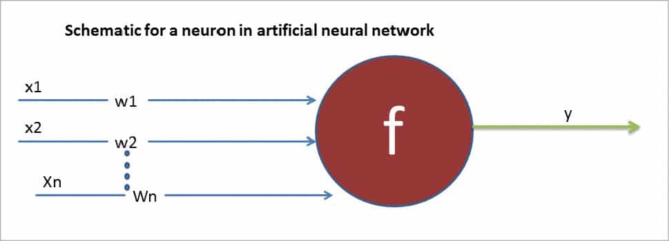
At its core, the neuron is optimised such that it receives information from other neurons and, in parallel, processes this information in a unique way, before sending the outcome (results) to other cells. This process works as shown in Figure 4.

Because of the advances mentioned earlier, humans are now able to simulate artificial neural networks using algorithms and computers. Each of the incoming connections is dynamically strengthened or weakened based on how many times it is used (this is also how humans learn new concepts). After being weighted by the strength of the respective connections, the inputs (Figure 5) are summed together in the cell body. This sum is then transferred to a new signal for other neurons to catch and analyse (this is called propagation along the cell’s axon and sent off to other neurons).

Using mathematical vector forms, this can be represented as follows:

Inputs as a vector X = [X1,X2 ….Xn]

And weights of the neuron as W = [W1, W2 …. Wn]

Therefore the output Y can be represented as Y = f(X.W + b)

Where “b” is the bias term.

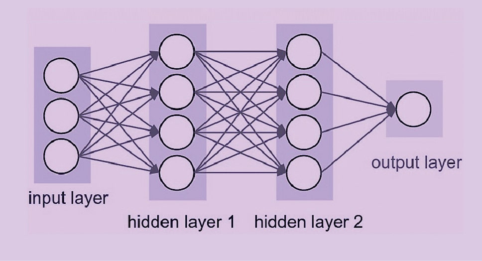
As such, many of these bunches of individual artificial neurons are connected together to form an ANN (artificial neural network). This ANN is a combo of various input and output layers along with hidden layers (as depicted in Figure 6).

Note 2: A hidden layer neuron is one whose output is connected to the inputs of other neurons and is therefore not visible as a network output (hence the term ‘hidden layer’).

Note 3: Refer to the article ‘Do deep nets really need to be deep?’ by Lei Jimmy Ba and Rich Caruana for more details.

Some time back, in 2014, it was observed that a training set with a huge data set in a shallow net, with one fully connected feed-forward hidden layer on the available data, yielded 86 per cent of the test data. But if this same data set was trained in a deeper neural net consisting of a convolutional layer, pooling layer, and three fully-connected feed-forward layers on the same data, 91 per cent accuracy on the same test set was obtained. This 5 per cent increase in accuracy of the deep net over the shallow net occurs because of the following reasons:

a) The deep net has more parameters.

b) The deep net can learn more complex functions, given the same number of parameters.

c) The deep net has better bias and learns more interesting/useful functions leading to invention and improvement of many algorithms.

A few algorithms

The scope of this article allows me to describe just a few important algorithms, based on these learnings and improvements. The following are the most used and popular algorithms. They are categorised as training feed-forward neural networks.

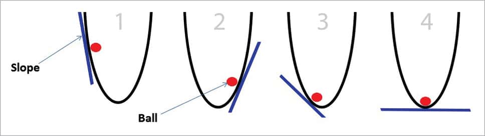
Gradient descent: Imagine there is a ball inside a bucket and the goal is to ‘get as low as possible’. This requires optimisation. In this case, the ball is optimising its position (left to right or right to left, based on the condition) to find the lowest point in the bucket.

The only information available is the slope of the side of the bucket at its current position, pictured with the blue line in Figure 7. Notice that when the slope is negative (downward from left to right), the ball should move to the right. However, when the slope is positive, the ball should move to the left. As you can see, this is more than enough information to find the bottom of the bucket in a few iterations. This is a sub-field of optimisation called gradient optimisation (gradient is just a fancy word for slope or steepness).

Note 4: To know more, you can refer to the article ‘Improving our neural network by optimising Gradient Descent’, posted by Iamtrask, better known as ‘Trask’.

The complexity of calculating the slope will become more and more challenging if, instead of a bucket, we have an uneven surface (like the surface of the moon or Mars). Getting the ball to the lowest position in this situation needs a lot of mathematical calculations and also more data sets.

Gradient descent isn’t perfect. There are some solutions around the corner that can help us to overcome these challenges, like:

a) Using multiple random starting states

b) Increasing the number of possible slopes and considering more neural networks

c) Using optimisations like ‘Native Gradient Descent’

d) Adding and tuning the alpha parameter

Note 5: What is alpha? As described above, the alpha parameter reduces the size of each iteration’s update in the simplest way possible.

Finally, gradient descent that uses non-linearities to solve the above problem is popular. Here, Sigmoidal neurons are used as training neurons.

The back-propagation algorithm: The back-propagation approach was pioneered by David E., Geoffrey Hinton and Ronald J. Sometimes we do not know what the hidden units are doing, but what we can do is compute how fast the error function changes as we change the hidden activity. With this we can find out how fast the error changes when we change the weight of an individual connection. Using this, we try to find the steepest descent.

Each hidden unit can affect many output units, and to compute the error derivatives for the activities of the layers below, we have to back-propagate to find the nearest values; hence, the name.

Stochastic and mini-batch gradient descent: There are three variants of gradient descent, which differ in how much data is used to compute the gradient of the objective function. Depending on the amount of data, one has to make a trade-off between the accuracy of the parameter update and the time it takes to perform an update. Instead of a single static error surface, by using a dynamic error surface and by descending on this stochastic surface, the ability to navigate flat regions improves significantly.

Note 6: Do refer to ‘An overview of gradient descent optimisation algorithms’ by Sebastian Ruder.

a) Batch gradient descent: Batch gradient descent (also known as Vanilla gradient descent) computes the gradient of the cost function with respect to the parameter θ for the entire training data set:

Θ=Θ—η.∇ΘJ(Θ)

b) Stochastic gradient descent: Stochastic gradient descent (SGD), in contrast, performs a parameter update for each training example — x(i) and label y(i):

Θ=Θ—η.∇ΘJ(Θ;x(i);y(i))

Batch gradient descent performs redundant computations for large data sets, as it recomputes gradients for similar examples before each parameter update. SGD does away with this redundancy by performing one update at a time. It is therefore usually much faster and can also be used to learn online.

c) SGD fluctuation: Batch gradient descent converges to the minimum point of the basin the parameters are placed in. On the one hand, SGD’s fluctuation enables it to jump to new and potentially better local minima, but on the other hand, this complicates convergence to the exact minimum, as SGD will keep overshooting. However, it has been shown that when we slowly decrease the learning rate, SGD shows the same convergence behaviour as batch gradient descent, almost certainly converging to a local or the global minimum for non-convex and convex optimisation, respectively.

Θ=Θ—η.∇ΘJ(Θ;x(i:i+n);y(i:i+n))

Note 7: Machine learning systems are mainly classified as supervised/unsupervised learning, semi-supervised learning, reinforcement learning, batch and online learning, etc. All these systems mainly work on training the data set. These broad categories are sub-divided into respective algorithms based on the training data set. A few popular examples are: k-nearest neighbours, linear and logistic regression, SVMs, decision trees and random forests, neural networks (RNN, CNN, ANN), clustering (k-means, HCA,), etc.

Open source support for deep learning

TensorFlow is an open source software library released in 2015 by Google to make it easier for developers to design, build and train deep learning models. Actually, TensorFlow originated as an internal library that Google developers used to build models in-house. Multiple functionalities were added later, as it became a powerful tool.

At a higher level, TensorFlow is a Python library that allows users to express arbitrary computation as a graph of data flows. Nodes in this graph represent mathematical operations, whereas edges represent data that is communicated from one node to another. Data in TensorFlow is represented as tensors, which are nothing but multi-dimensional arrays (from 1D tensor, 2D tensor, 3D tensor…etc.). The TensorFlow library can be downloaded straight away from https://www.tensorflow.org/.

There are many other popular open source libraries that have popped up over the last few years for building neural networks. These are:

1) Theano: Built by the LISA lab at the University of Montreal (https://pypi.python.org/pypi/Theano)

2) Keras (https://pypi.python.org/pypi/Keras)

3) Torch: Largely maintained by the Facebook AI research team (http://torch.ch/)

All these options boast of a sizeable developer community, but of all these TensorFlow stands out because of its features such as the shorter data training time, ease of writing and debugging code, availability of many classes of models, and multiple GPU support on a single machine. Also, it is well suited for production-ready use cases.

Deep learning has become an extremely active area of research and is finding many applications in real life challenges. Companies such as Google, Microsoft and Facebook are actively forming deep learning teams in-house. The coming days will witness more advances in this field— agents capable of mastering Atari games, driving cars, trading stocks profitably and controlling robots.