


We have now arrived at the fifth article in our series on SageMath. Recall that SageMath follows Python 3 syntax. Thus, effectively, SageMath is Python on steroids, offering all the power of Python with the additional kick from SageMath specific methods and utilities. We ended the last article in this series with a discussion of directed graphs, yet another variant of graphs that is extremely useful in handling many real-world scenarios. We will begin this article by continuing our discussion on directed graphs and then move on to directed multigraphs.
Before we begin, let us answer the two questions I posed in the last article in this series. The first question: How many edges does a complete directed graph on 10 vertices have? First, let us find the answer mathematically. There are 10 vertices, and each vertex has a directed edge to the 9 other vertices. Notice that, for each pair of vertices, there are two directed edges (one in each direction). Thus, the total number of directed edges in a complete directed graph on 10 vertices is 10 x 9 = 90. Now, let us verify this answer by executing SageMath code. Upon executing the following line of code on CoCalc, we get the answer as 90, the same as the one we found mathematically.
digraphs.Complete(10).size( )
Now, the second question: How many edges are there in an undirected complete graph with 10 vertices? First, let us find the answer mathematically. There are 10 vertices, and each vertex can connect to 9 other vertices. However, since each edge is counted twice (once from each vertex of the pair), we divide by 2 to get the correct number of unique edges. Hence, the number of edges in an undirected complete graph on 10 vertices is (10 x 9) / 2 = 45. Now, let us verify this answer by executing SageMath code. Upon executing the following line of code on CoCalc, we get the answer as 45, the same as the one we found mathematically.
graphs.CompleteGraph(10).size( )
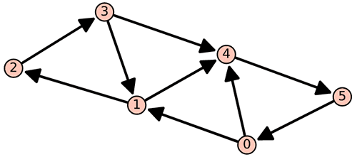
Now, let us generate a slightly more complex directed graph for detailed analysis. The program ‘dgraph12.sagews’ shown below generates a directed graph called Dgraph_12.
DG = DiGraph( )
DG.add_vertices([0, 1, 2, 3, 4, 5])
DG.add_edges([(0, 1), (0, 4), (1, 2), (1, 4), (2, 3), (3, 1), (3, 4), (4, 5), (5, 0)])
DG.show( )
The code does not need any explanation, as it is similar to the directed graphs we have generated in the previous article in this series. Upon executing the program ‘dgraph12.sagews’ using CoCalc, we obtain the graph called Dgraph_12, which is shown in Figure 1.
Now, let us see how the adjacency matrix of a directed graph looks. To do this, add the following line of code at the end of the program called ‘dgraph12.sagews’.
DG.adjacency_matrix( )
Upon executing the modified program, the following adjacency matrix will also be displayed on the screen.
[0 1 0 0 1 0]
[0 0 1 0 1 0]
[0 0 0 1 0 0]
[0 1 0 0 1 0]
[0 0 0 0 0 1]
[1 0 0 0 0 0]
The adjacency matrix shown above represents a directed graph with 6 vertices and, hence, is a 6 x 6 matrix. Each entry at position (i, j) in the matrix indicates whether there is a directed edge from vertex i to vertex j. An entry of 1 indicates that there is a directed edge from vertex i to vertex j, while an entry of 0 indicates that there is no directed edge from vertex i to vertex j. For example, row 0 indicates that vertex 0 has directed edges to vertex 1 and vertex 4. Furthermore, it can be observed that information about the edges incident on vertex 0 is not provided by this row of the adjacency matrix. For example, the information regarding the edge from vertex 5 to vertex 0 is provided by the row corresponding to vertex 5.
Now, let us see how the incidence matrix of a directed graph looks. To do this, add the following line of code at the end of the program called ‘dgraph12.sagews’.
DG.incidence_matrix( )
Upon executing the modified program, the following incidence matrix will also be displayed on the screen.
[-1 -1 0 0 0 0 0 0 1]
[ 1 0 -1 -1 0 1 0 0 0]
[ 0 0 1 0 -1 0 0 0 0]
[ 0 0 0 0 1 -1 -1 0 0]
[ 0 1 0 1 0 0 1 -1 0]
[ 0 0 0 0 0 0 0 1 -1]
The incidence matrix shown above represents the directed graph Dgraph_12 with 6 vertices and 9 edges. Each row in the incidence matrix indicates a vertex, so there are 6 rows denoting vertices 0 to 5. Each column in the incidence matrix indicates an edge, so there are 9 columns denoting the 9 edges. In each column, an entry of -1 denotes the starting vertex and an entry of 1 denotes the ending vertex of that particular edge. For example, column 2 represents the edge from vertex 0 to vertex 4, which starts at vertex 0 (represented by -1) and ends at vertex 4 (represented by 1).
When we discussed undirected graphs, we came across connected graphs in which there are paths between any pair of vertices. There is a related concept in directed graphs called strongly connected directed graphs. A strongly connected directed graph is a directed graph in which there exists a directed path between any pair of vertices. Recall that, unlike undirected graphs, the existence of a path (directed) from vertex A to vertex B does not guarantee a path (directed) from vertex B to vertex A. An orientation of an undirected graph is a directed graph in which every original undirected edge is given one of the two possible orientations. A very interesting research topic in graph theory is the study of orientations of undirected graphs that result in strongly connected directed graphs—a topic of great interest to me, as my research in this area enabled me to obtain a PhD from IIT Palakkad.
Let us see how a strongly connected directed graph can be obtained from an undirected graph by introducing yet another highly useful SageMath method used to generate random graphs. A random graph is a graph where properties like the number of vertices, edges, and connections between them are determined randomly. In simpler terms, it is a graph generated by a random process, such as tossing a coin to decide whether to include an edge between a pair of vertices. Random graphs are used to model real-world networks such as social networks, biological networks, etc. Now, consider the code below, which uses the SageMath method called RandomGNP( ) to generate a random graph.
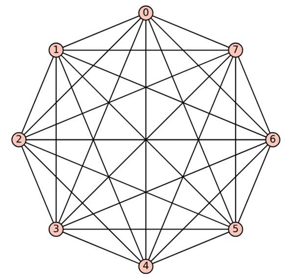
rgraph = graphs.RandomGNP(8, 1)
rgraph.show( )
Execute the above line of code several times on CoCalc and observe the graphs each time. You will see that the code always generates the same graph (an undirected complete graph on 8 vertices), as shown in Figure 2. Why does this happen instead of producing distinct graphs each time? To answer this, we need to understand the purpose of the two input parameters given to the method RandomGNP( ). The first parameter defines the number of vertices in the randomly generated graph (8 in this case). The second parameter defines the probability with which an edge is created between each pair of vertices, with a range between 0 and 1, inclusive. In the example above, the probability is set to 1, resulting in a 100% chance of generating an edge between each pair of vertices. Thus, an edge is created between every pair of vertices, leading to the generation of a complete graph. What graph will be displayed if the method RandomGNP( ) is called as: ‘graphs.RandomGNP(8, 0)’? Please give it a try before you proceed any further. I will provide the answer at the end of this article.
Now, let us change the second parameter so that the probability of creating an edge between each pair of vertices is 0.3. The program ‘rgraph13.sagews’ shown below generates a random graph (line numbers have been included for clarity in the explanation).
1. rgraph = graphs.RandomGNP(8, 0.3)
2. rgraph.show( )
3. sgraph = rgraph.strong_orientation( )
4. sgraph.show( )
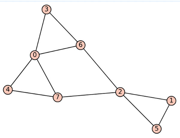
Now, let us go through the code for better understanding. Line 1 creates a random undirected graph rgraph using the RandomGNP( ) method from SageMath’s graphs library. The first parameter, 8, specifies the number of vertices in the graph. The second parameter, 0.3, specifies the probability of edge creation between any pair of vertices. Line 2 displays the random graph generated. Figure 3 shows a random graph called Rgraph_13 generated in one of the executions of the above code. Keep in mind that the graph generated with each execution of the code will almost certainly be different from the one generated previously. Also, the chances of you getting a graph isomorphic to Rgraph_13 are near zero.
Line 3 of the code converts the undirected graph rgraph into a directed graph sgraph using the strong_orientation( ) method. Recall that a strong orientation of a graph is a directed graph in which each undirected edge is given a direction such that the resulting directed graph is strongly connected. A strongly connected directed graph has a directed path from any vertex to any other vertex. Finally, Line 4 displays the strongly oriented directed graph sgraph, shown in Figure 4, with its vertices and directed edges.
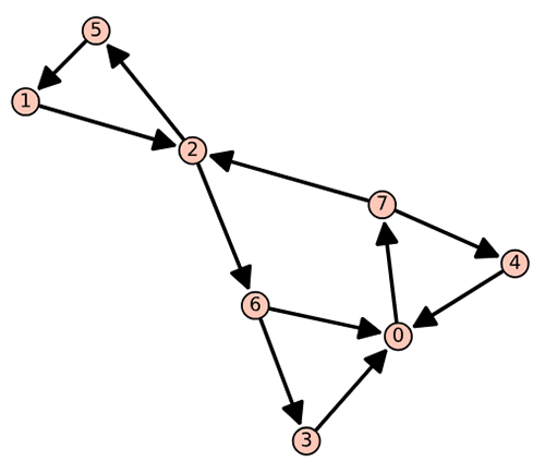
An important question is: when can an undirected graph have an orientation such that the resulting directed graph is strongly connected? An important theorem by the famous mathematician Robbins proved that every 2-edge connected graph can have a strongly connected directed graph. A graph is said to be 2-edge connected if it remains connected even if any one edge is removed. If the given graph is not 2-edge connected, the orientation returned by the strong_orientation( ) method will ensure that each 2-edge connected component has a strongly connected orientation. Please verify that there is a directed path between every pair of vertices in Rgraph_13, shown in Figure 4, before you proceed further.
In the last two articles in this series, we dealt with undirected multigraphs. Similarly, there are directed multigraphs in which multiple directed edges can exist between a pair of vertices. Let us now see an example of directed multigraphs. The program ‘dmultigraph14.sagews’ shown below generates a directed multigraph called Dmultigraph_14.
dirmg = DiGraph(multiedges=True, loops=True)
dirmg.add_vertices([0, 1, 2, 3])
edges = [(0, 1), (0, 1), (1, 2), (1,3), (2, 3), (2, 2), (3, 0), (3, 1)]
dirmg.add_edges(edges)
dirmg.show(edge_labels=False)
Upon executing the program ‘dmultigraph14.sagews’ using CoCalc, we obtain a directed multigraph called Dmultigraph_14, which is shown in Figure 5. From Figure 5, it can be observed that there are two edges between vertices 1 and 3 (one from vertex 1 to vertex 3 and the other from vertex 3 to vertex 1), as well as two edges between vertices 0 and 1 (both directed from vertex 0 to vertex 1).
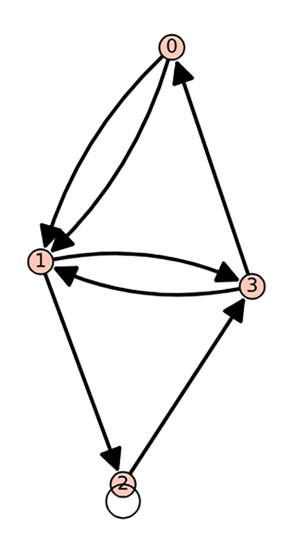
multigraph Dmultigraph_14
Now, let us revisit the examples we have discussed to understand the use of undirected and directed graphs in modelling real-world scenarios. We used undirected graphs to represent a city street map where all the roads allow two-way transportation and directed graphs to represent a city street map where all the roads allow only one-way traffic. However, in reality, no city has such a uniform road system. Every city has some roads that allow two-way traffic and others that only allow one-way traffic. How can we capture the features of such a city street map and use graph-theoretic methods to elicit information? Mixed graphs and mixed multigraphs are handy in this scenario. Mixed graphs and mixed multigraphs can have both directed and undirected edges. In the example of the city street map, the undirected edges will represent roads that allow two-way traffic, and the directed edges will represent roads that allow only one-way traffic.
However, we face a slight hiccup when using SageMath to simulate mixed graphs and mixed multigraphs. The problem is that SageMath does not have a built-in class to handle mixed graphs and mixed multigraphs directly. Instead, we can use directed multigraphs to simulate mixed graphs and mixed multigraphs, which allow parallel directed edges. This is helpful because an undirected edge between vertices, say A and B, is equivalent (for almost all practical purposes) to two directed edges: one from vertex A to vertex B and another from vertex B to vertex A. This double directed edge construction is a classical technique used in graph theory to construct mixed graphs and mixed multigraphs using directed multigraphs.
Let us see a practical example of representing a mixed graph with a directed multigraph. How can we represent the mixed graph with four vertices shown in Figure 6 using a directed multigraph?
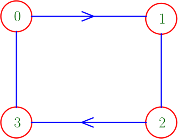
The program ‘dmultigraph15.sagews’ shown below generates a directed multigraph called Dmultigraph_15, which simulates the mixed graph shown in Figure 6.
DG = DiGraph( )
DG.add_vertices([0, 1, 2, 3])
edges = [(0, 1), (1, 2), (2, 1), (2, 3), (3, 0), (0, 3)]
DG.add_edges(edges)
DG.show( )
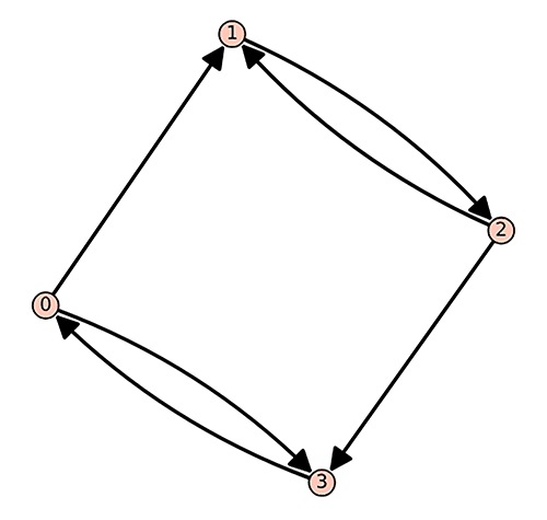
Upon executing the program ‘dmultigraph15.sagews’ using CoCalc, we obtain a directed multigraph called Dmultigraph_15, which is shown in Figure 7. Observe Figure 7 carefully and verify that Dmultigraph_15 indeed simulates the mixed graph shown in Figure 6. Also, keep in mind that to simulate mixed multigraphs, we can use directed multigraphs with multiple directed edges in the same direction, like the two directed edges from vertex 0 to vertex 1 in Dmultigraph_14 shown in Figure 5. Try to draw a mixed multigraph and then simulate it using a directed multigraph as an exercise.
Now, it is time to wrap up our discussion. First, let me answer the question I posed earlier. The line of code ‘rgraph = graphs.RandomGNP(8, 0)’ will generate a graph with 8 isolated vertices and 0 edges, regardless of how many times you execute it. This happens because the probability of edge creation is zero, as the second parameter provided is 0.
In this article also, we have explored some important types of graphs that can be used to analyse real-world scenarios. Keep in mind that there are many other complex graph variants that can be used to explore even more intricate real-world situations. However, those are beyond the scope of this series, in which our focus is on undirected graphs, directed graphs, multigraphs, mixed graphs, and mixed multigraphs. In the next article in this series, we will delve into several key graph-theoretic methods and topics before concluding our discussion on graph theory and moving on to other mathematical topics of interest.


