


We continue our journey of learning SageMath, a very powerful tool that will be a crucial weapon in our arsenal in a world soon to be dominated by AI, machine learning, and data science.
In the past few articles in this series we discussed our first mathematical topic of great interest: graph theory. Specifically, we explored undirected simple graphs, both theory and practical coding. By the end of the third article in this series (published in the July 2024 issue of OSFY), we began focusing our attention on another important class of graphs: undirected multigraphs. We will resume our discussion from where we left off. Please refer to the program ‘mgraph7.sagews’ and the multigraph Mgraph_7 (Figure 5) generated by this program, given in the previous article in this series, before proceeding further with this article for a clear understanding. Recall that we also had a detailed discussion about the differences between undirected simple graphs and multigraphs in the previous article. Furthermore, any theoretical concept not elaborately explained in this article is discussed in detail in one of the previous articles.
The plan is to test every method we tested on the undirected simple graphs we generated using SageMath in the previous articles on Mgraph_7. By doing this, we will know which method does not work for undirected multigraphs and how they behave if they do work. First, let us print the adjacency matrix of the undirected multigraph Mgraph_7. To do that, add the following line of code at the end of the program called ‘mgraph7.sagews’.
print(MG.adjacency_matrix( )) |
As before, we use the online tool called CoCalc to execute the modified program. Upon execution of the modified program, the following additional output will be displayed on the screen. But how is it different from the adjacency matrix of an undirected simple graph?
[1 2 0 2][2 1 2 0][0 2 1 2][2 0 2 1] |
First, the adjacency matrix of an undirected simple graph only contained 0s or 1s as entries, indicating that there could be at most one edge between any pair of vertices. However, in the adjacency matrix shown above, we also have 2s, indicating that there are 2 parallel edges between certain pairs of vertices in the undirected multigraph Mgraph_7. Notice that there can be any number of edges between a pair of vertices in an undirected multigraph, and hence the corresponding adjacency matrix can contain any number greater than or equal to 0. Second, the diagonal elements of the adjacency matrix of an undirected simple graph contain only 0s, indicating that such graphs do not contain any loops. In contrast, the diagonal elements of the adjacency matrix of the undirected multigraph Mgraph_7 also have 1s, indicating that vertices corresponding to such entries have loops. Also, keep in mind that a vertex of an undirected multigraph can have more than one loop, and hence the diagonal entry corresponding to such vertices in the adjacency matrix can have entries greater than 1.
Now, let us print the incidence matrix of the undirected multigraph Mgraph_7. To do that, add the following line of code at the end of the program called ‘mgraph7.sagews’.
print(MG.incidence_matrix( )) |
Upon execution of the modified program, the following additional output will be displayed on the screen. But how is it different from the incidence matrix of an undirected simple graph?
[2 1 1 1 1 0 0 0 0 0 0 0][0 1 1 0 0 2 1 1 0 0 0 0][0 0 0 0 0 0 1 1 2 1 1 0][0 0 0 1 1 0 0 0 0 1 1 2] |
Well, the incidence matrix of an undirected simple graph only contains 0s or 1s as entries. Furthermore, since every edge has exactly two endpoints, every column of the incidence matrix will have exactly two 1s. However, in the incidence matrix shown above, we also have 2s, indicating the presence of loops in certain vertices in the undirected multigraph Mgraph_7. For example, in Mgraph_7, columns 1, 6, 9, and 12 correspond to edges that are loops. When there are parallel edges in an undirected multigraph, the columns corresponding to these edges are duplicates of each other. So, in Mgraph_7, columns 2 and 3, 4 and 5, 7 and 8, and 10 and 11 are duplicates of each other. Also, notice that the sum of the entries in a column in the incidence matrix is still 2, since an edge only has two endpoints, whether it is a loop, a single edge, or multiple edges (parallel edges).
Now, let us find all the paths between a pair of vertices in an undirected multigraph. Add the following line of code at the end of the program called ‘mgraph7.sagews’ to find all the paths between vertices 2 and 4 in Mgraph_7.
print(MG.all_paths(2, 4)) |
Upon execution of the modified program, the following additional output will be displayed on the screen.
[[2, 1, 4], [2, 3, 4]] |
Notice that only distinct paths through different vertices are shown in the output. The method all_paths( ) completely ignores the presence of loops and multiple edges in the undirected multigraph Mgraph_7.
Now, let us test the longest_cycle( ) method on the undirected multigraph Mgraph_7. When used on an undirected simple graph, this method gives the length of the longest cycle. Add the following line of code at the end of the program called ‘mgraph7.sagews’ to test this method on an undirected multigraph.
MG.longest_cycle( ) |
Upon execution of the modified program, we get the following error message displayed on the screen. Why do we get this error?
ValueError: This method is not known to work on graphs with multiedges/loops. Perhaps this method can be updated to handle them, but in the meantime if you want to use it please disallow multiedges/loops using allow_multiple_edges( ) and allow_loops( ). |
Well, this is because the longest_cycle( ) method in SageMath does not support graphs with loops or multiple edges. A workaround for this limitation is to create a new graph without loops and multiple edges from the original graph and then find the longest cycle in this new graph. However, be careful when using this hack because there are multiple definitions for the term ‘cycle’ in graph theory. I urge you to read the Wikipedia article titled ‘Cycle (graph theory)’ for further details. Wikipedia considers a cycle and a circuit as two distinct entities, with every cycle also being a circuit. However, many graph theorists consider a cycle to be equivalent to a circuit (according to the Wikipedia definition), a broader class of graphs. Also, note that the method longest_cycle( ), whether called as MG.longest_cycle(induced=True) or MG.longest_cycle(induced=False), will also lead to an error when used with undirected multigraphs.
Now, let us check whether the undirected multigraph Mgraph_7 contains an Eulerian circuit. To do that, add the following line of code at the end of the program called ‘mgraph7.sagews’.
MG.eulerian_circuit(labels=False) |
Upon execution of the modified program, the following additional output will be displayed on the screen. This clearly indicates that the undirected multigraph Mgraph_7 has an Eulerian circuit. Please refer to Figure 5 in the previous article and verify that this indeed is an Eulerian cycle.
[(1, 4), (4, 4), (4, 3), (3, 3), (3, 2), (2, 2), (2, 3), (3, 4), (4, 1), (1, 2), (2, 1), (1, 1)] |
Now, let us check whether the undirected multigraph Mgraph_7 contains a Hamiltonian circuit. To do that, add the following line of code at the end of the program called ‘mgraph7.sagews’.
MG.hamiltonian_cycle( ) |
Upon execution of the modified program, we get an error message displayed on the screen. The issue again stems from the loops and multiple edges present in our graph Mgraph_7. The hamiltonian_cycle( ) method has problems handling loops and multiple edges. The fix is the same as before — create a new graph without loops and multiple edges from the original graph, and then check for a Hamiltonian cycle in this new graph. This time the answer will be accurate. If an undirected simple graph has a Hamiltonian cycle, then the same Hamiltonian cycle will be present even if we add multiple edges and loops. In general, if a graph has a Hamiltonian cycle, it will continue to have that cycle even if we add more edges. However, the same is not true about Eulerian cycles in a graph. Please think about some examples to verify that the statement I made is indeed true.
The SageMath methods we discussed just now clearly indicate that we must be careful when dealing with multigraphs. Methods that work for simple graphs may not work for multigraphs. However, with SageMath being free and open source software, you can edit the source code to create methods that suit your needs once you gain sufficient mastery.
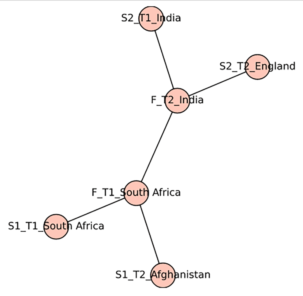
Now, it is time for us to familiarise ourselves with one more type of undirected simple graph: the tree. A tree is a graph without any cycles. Trees can also be used to represent many real-world scenarios and problems. For example, the knockout stage of any sports tournament can be represented using a tree. The program ‘tree8.sagews’ shown below generates a tree called the Tree_8.
T = Graph( )teams = [‘S1_T1_South Africa’, ‘S1_T2_Afghanistan’, ‘S2_T1_India’, ‘S2_T2_England’, ‘F_T1_South Africa’,’F_T2_India’]T.add_vertices(teams)T.add_edges([(‘S1_T1_South Africa’, ‘F_T1_South Africa’),(‘S1_T2_Afghanistan’, ‘F_T1_South Africa’),(‘S2_T1_India’, ‘F_T2_India’),(‘S2_T2_England’, ‘F_T2_India’),(‘F_T1_South Africa’, ‘F_T2_India’)])T.plot(vertex_size=600).show( ) |
The code does not need any explanation, as it is similar to the other undirected simple graphs generated earlier in this series. The only difference is that this graph does not contain any cycles. In the last line of the code, we use the plot( ) method to provide the option vertex_size so that larger vertices are displayed by the show( ) method. Upon execution of the program ‘tree8.sagews’, we get the graph called tree_8 shown in Figure 1. Notice that this is the knockout stage (semifinals and final) of the recently concluded 2024 ICC Men’s T20 World Cup. To view a tree with a larger number of vertices, see the Wikipedia page of the 2024 Wimbledon tennis championship. A family tree is another example where a tree can be used to capture real-world information.
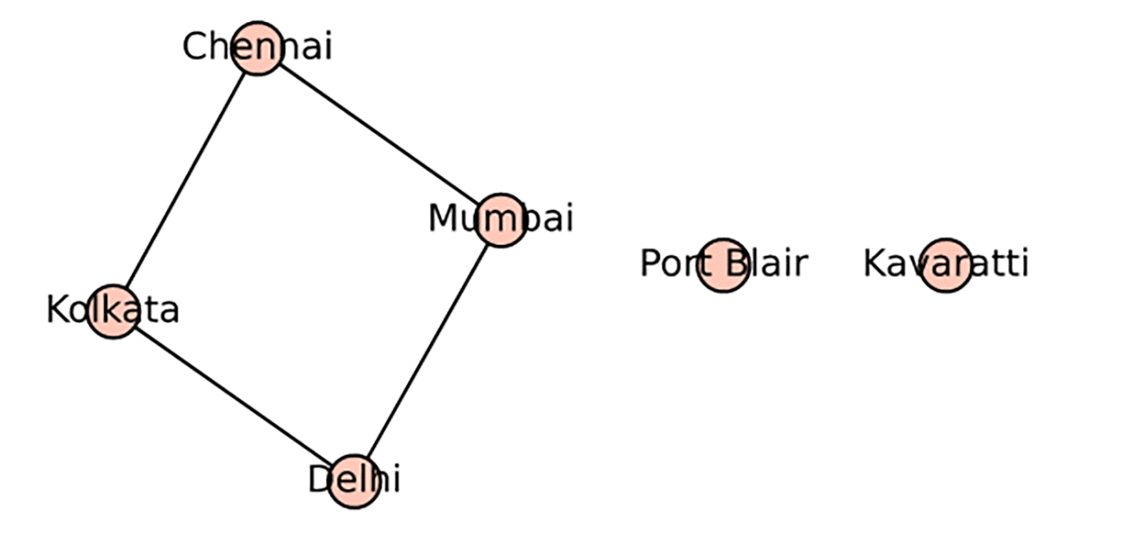
Before we move on from undirected graphs (simple or multigraphs), we need to familiarise ourselves with two more graph-theoretic terms: connected and disconnected graphs. So far, we have only encountered connected graphs in this series. A connected undirected graph is a graph in which there is a path between every pair of vertices. Use the method all_paths( ) offered by SageMath to verify the existence of at least one path between any pair of vertices in all the graphs we have discussed so far in this series. On the other hand, a disconnected graph is a graph that is not connected. In such a graph, there is at least one pair of vertices that has no path connecting them. The program ‘disgraph9.sagews’ shown below generates a graph called Disgraph_9, which shows the rail connectivity between several cities/towns in India.
G = Graph( )G.add_vertices([‘Mumbai’, ‘Delhi’, ‘Chennai’, ‘Kolkata’, ‘Port Blair’, ‘Kavaratti’])G.add_edges([(‘Mumbai’, ‘Delhi’),(‘Delhi’, ‘Kolkata’),(‘Kolkata’, ‘Chennai’),(‘Chennai’, ‘Mumbai’)])G.show( ) |
This code also does not need any explanation, as it is similar to the other undirected simple graphs generated earlier in this series. Upon execution of the program ‘disgraph9.sagews’, we get the graph called Disgraph_9 shown in Figure 2. This graph shows the rail connectivity between Delhi, Mumbai, Kolkata, Chennai, Kavaratti (the capital of the union territory of Lakshadweep), and Port Blair (the capital of the union territory of the Andaman and Nicobar Islands). Keep in mind that Disgraph_9 only represents connectivity between places and not the actual geographical location of these places on the map of India. We all know that a person can travel by train between Delhi, Mumbai, Kolkata, and Chennai. However, since Kavaratti and Port Blair are located on islands, there is no rail connectivity to those cities from other cities in India. In situations like this, disconnected graphs are very useful for capturing essential data from real-world scenarios.
Let us also familiarise ourselves with some connectivity-related methods available in SageMath. To do that, add the following lines of code at the end of the program called ‘disgraph9.sagews’.
G.is_connected( )G.connected_components_number( )G.connected_components(sort=True)G.connected_components_sizes( )G.all_paths(‘Delhi’, ‘Mumbai’)G.all_paths(‘Delhi’, ‘Port Blair’) |
Upon execution of the modified program, the following additional output will be displayed on the screen.
False3[[‘Chennai’, ‘Delhi’, ‘Kolkata’, ‘Mumbai’], [‘Port Blair’], [‘Kavaratti’]][4, 1, 1][[‘Delhi’, ‘Mumbai’], [‘Delhi’, ‘Kolkata’, ‘Chennai’, ‘Mumbai’]][ ] |
Now, let us compare the code and the corresponding output for better understanding. The method G.is_connected( ) checks if the graph G is connected. Since the graph Disgraph_9 is not connected, the answer is given as False. The method G.connected_components_number( ) returns the number of connected components in the graph G. Since Delhi, Mumbai, Kolkata, and Chennai are connected with each other, they form one connected component. Kavaratti and Port Blair are located on islands, forming two more components. Hence, the answer is 3. The method G.connected_components(sort=True) returns the connected components of the graph G. The parameter sort=True ensures that the vertices inside each component are sorted according to the default ordering. From the output, we can see that the list has three elements, each containing the names of the connected components.
The method G.connected_components_sizes( ) returns the sizes of the connected components in the graph G. The size indicates the number of vertices in a particular connected component. Comparing with the previous output, we can see that the output [4, 1, 1] is correct. The method call G.all_paths(‘Delhi’, ‘Mumbai’) returns all possible paths between the vertices ‘Delhi’ and ‘Mumbai’ in the graph G. The list shows the direct path from ‘Delhi’ to ‘Mumbai’ as well as the indirect path through vertices ‘Kolkata’ and ‘Chennai’. Similarly, the method call G.all_paths(‘Delhi’, ‘Port Blair’) returns all paths between vertices ‘Delhi’ and ‘Port Blair’ if they exist. Since there is no path between ‘Delhi’ and ‘Port Blair’, this method call returns an empty list, as you can observe in the output above.
Now, let us move on to the next type of graph, the directed graph (also known as a digraph). But why do we need directed graphs? We already have undirected simple graphs and multigraphs, along with a number of powerful methods to elicit information from them. Well, the reason is that undirected graphs (simple and multigraphs) can only represent symmetric relationships between two entities or objects. Let us consider the example we discussed in the second article in this series, available on the OSFY portal at ‘https://www.opensourceforu.com/2024/03/sagemath-demystifying-graphs’. In the example, we used an undirected graph to capture the friendship between six people. An edge between a pair of vertices indicates that they are friends with each other. However, human relationships do not always work this way. What if I am in love with somebody and she doesn’t care about me at all? Well, an undirected graph cannot represent such a relationship effectively.
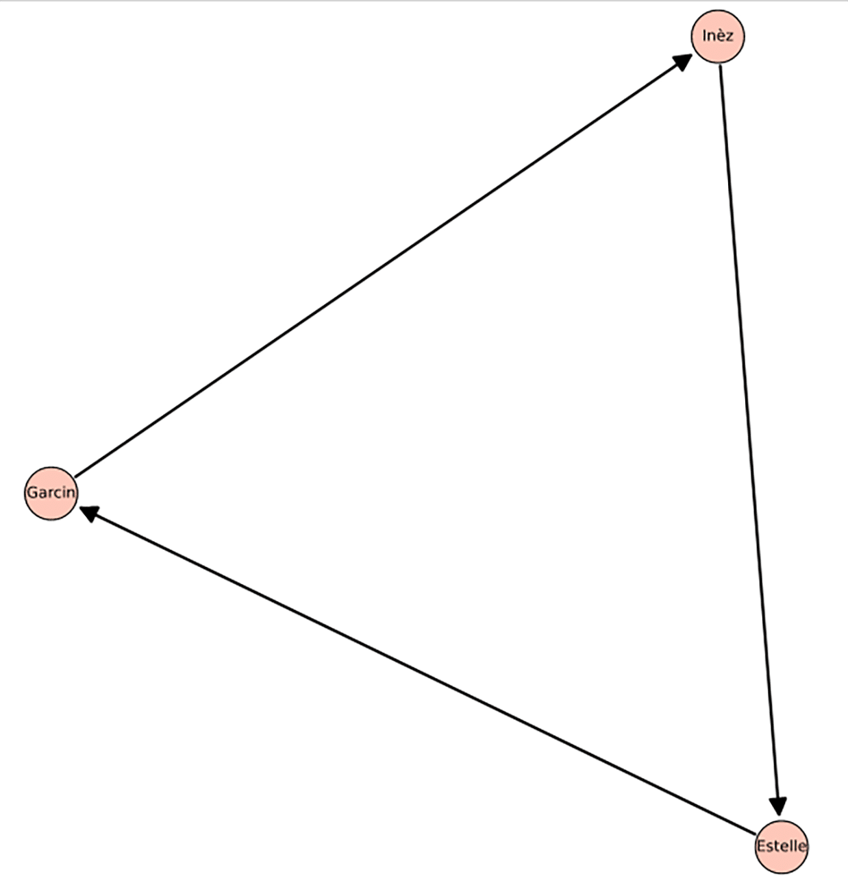
Let us use three characters from the world-famous play ‘No Exit’, written by Jean-Paul Sartre, a renowned philosopher and writer (a Nobel Laureate in literature and the only person who voluntarily declined the prize, true to his existentialist philosophy). In this play, three people — Inèz, Estelle, and Garcin — are condemned to hell for eternity for their sins. They are the only inhabitants of a room in hell where they expect torture. However, there is no physical torture, and after some time, Inèz becomes attracted to Estelle, Estelle becomes attracted to Garcin, and Garcin becomes attracted to Inèz. Thus, everyone is in love but not loved in return for eternity, which is the real torture. Eventually, they come to believe that “Hell is other people” (Sartre’s somewhat infamous quote, which, of course, nobody should take literally). Now, let us use a directed graph to denote the relationships between the three characters in the play. The program ‘dgraph10.sagews’ shown below generates a graph called Dgraph_10 (line numbers have been included for clarity in the explanation).
1. DG = DiGraph( )2. DG.add_vertices([‘Inèz’, ‘Estelle’, ‘Garcin’])3. DG.add_edges([(‘Inèz’, ‘Estelle’), (‘Estelle’, ‘Garcin’), (‘Garcin’, ‘Inèz’)])4. DG.plot(vertex_size=1200, figsize=[8, 8]).show( ) |
Now, let us go through the code for better understanding. Line 1 initialises an empty directed graph DG using SageMath’s DiGraph class. Line 2 adds three vertices to the graph: ‘Inèz’, ‘Estelle’, and ‘Garcin’. These vertices represent the three characters in the play ‘No Exit’. Line 3 adds three directed edges to the graph: an edge from ‘Inèz’ to ‘Estelle’, an edge from ‘Estelle’ to ‘Garcin’, and an edge from ‘Garcin’ to ‘Inèz’. These edges represent the unreciprocated feelings between the three characters. Line 4 plots the directed graph DG. The parameter vertex_size=1200 sets the size of the vertices in the plot, and the parameter figsize=[8, 8] sets the size of the plot to 8 x 8 inches. Finally, the show( ) method displays the plot. Upon execution of the program ‘dgraph10.sagews’, we get the graph called Dgraph_10. The directed graph Dgraph_10, where the directed edges visually depict the direction of each character’s attraction towards another, is shown in Figure 3.
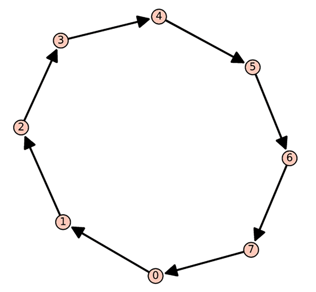
Now, let us generate a directed cycle of length 8 using SageMath. We will use this cycle to learn an important difference between a directed graph and an undirected graph. The program ‘dcycle11.sagews’ shown below generates a graph called Dcycle_11.
DG = DiGraph( )DG.add_vertices([0, 1, 2, 3, 4, 5, 6, 7])DG.add_edges([(0, 1), (1, 2), (2, 3), (3, 4), (4, 5), (5, 6), (6, 7), (7, 0)])DG.show( ) |
The code does not need any explanation, as it is similar to the previous directed graph we have generated. Upon execution of the program ‘dcycle11.sagews’, we get the graph called Dcycle_11, which is shown in Figure 4.
Now, it is time for us to better understand the main difference between undirected and directed graphs. As seen in the first example, we can represent asymmetric relationships using directed graphs. To illustrate this point further, let us use the distance( ) method offered by SageMath. This method finds the distance between two vertices. Recall that the distance between a pair of vertices is the number of edges in the shortest path between those two vertices. First, let us test the distance( ) method on the undirected graph Disgraph_9. To do that, add the following lines of code at the end of the program called ‘disgraph9.sagews’.
G.distance(‘Kolkata’, ‘Mumbai’)G.distance(‘Mumbai’, ‘Kolkata’)G.distance(‘Mumbai’, ‘Kavaratti’) |
Upon execution of the modified program, the following additional output will be displayed on the screen.
22+Infinity |
From the output, it is clear that the distance from ‘Kolkata’ to ‘Mumbai’ and ‘Mumbai’ to ‘Kolkata’ is the same (2), thus showing the symmetric nature of undirected graphs. Use the distance( ) method on the undirected graphs we have generated in the previous articles to test that the distance between any pair of vertices is the same in both directions. Furthermore, the distance from ‘Mumbai’ to ‘Kavaratti’ is defined as infinity because there is no path between ‘Mumbai’ and ‘Kavaratti’.
Now, let us test the distance( ) method on the directed graph Dcycle_11. To do that, add the following lines of code at the end of the program called ‘dcycle11.sagews’.
DG.distance(1, 3)DG.distance(3, 1) |
Upon execution of the modified program, the following additional output will be displayed on the screen.
26 |
The output shows that the distance from vertex 1 to 3 is 2, while the distance from vertex 3 to 1 is 6, demonstrating the asymmetric nature of directed graphs.
It is worth noting that SageMath, as mentioned earlier, offers special methods for generating various graphs, both undirected and directed. For example, in the first article in this series, we generated a graph known as the icosahedral graph. Similarly, SageMath provides a method called Circuit( ) to generate directed cycles. Upon execution of the following line of code on CoCalc, we get a directed cycle of length 8 isomorphic to the directed cycle Dcycle_11.
digraphs.Circuit(8).show( ) |
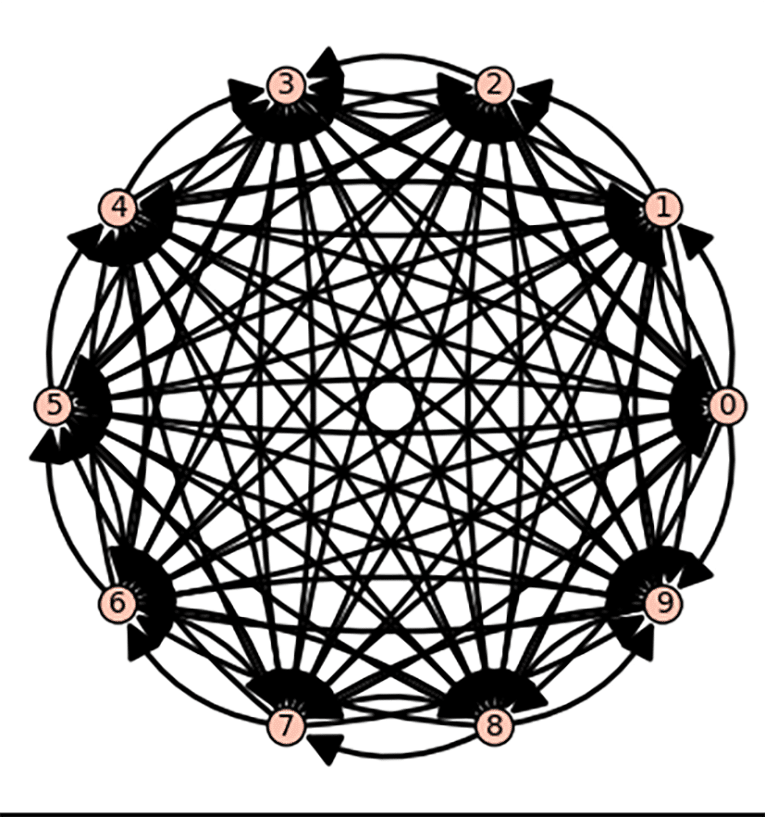
Let us see one more example. Execute the following line of code on CoCalc to generate a complete directed graph. This type of graph has a directed edge from every vertex to every other vertex.
digraphs.Complete(10).show( ) |
Upon executing the above line of code, we obtain a complete directed graph on 10 vertices, shown in Figure 5. How many edges does this graph have? Please find the answer both mathematically and by executing SageMath code. Additionally, undirected complete graphs (often simply called complete graphs) also exist. How many edges are there in an undirected complete graph with 10 vertices? All these questions will be answered in the next article in this series.
In this article, we conducted a thorough investigation of undirected simple graphs as well as multigraphs. We were also introduced to directed graphs, but there is still much more to learn about them. Additionally, we need to discuss mixed graphs and mixed multigraphs, yet another variant. Hence, we will be discussing more about graphs in the next few articles of this series as well.
A small side note: I am finding it increasingly difficult to give meaningful titles to the articles as we delve deeper into exploring graphs extensively. However, let me assure you that it is absolutely essential to do so. As social media explodes, information floods in, and AI takes centre stage, graphs will become crucial tools to understand and make sense of it all. So, in the next article, we will explore many more powerful graph-theoretic methods offered by SageMath. Until then, goodbye.


