Julia is an emerging star in the world of programming languages. It offers the coveted combination of high performance and productivity. What Julia offers in terms of execution speed may almost seem unbelievable, especially to newcomers to this language. This article provides an introduction to Julia, which is as simple as Python to learn, and on par with C and Fortran in terms of execution speed.
As a programmer you may question the very need for yet another programming language. Such a question is very fair with the available ecosystem of a few hundred languages. However, each programming language is designed to achieve a specific goal. So it would be right to start this article by stating the specific objective of designing the Julia language. There is a basic conundrum in programming: execution speed vs development ease. If a language leans towards programmers, then there are likely to be issues with the execution speed. On the other hand, if you want to generate optimised code, then the development process will probably be harder. For example, a system completely designed in C programming language will generate optimal assembly code. However, development of such a system would take longer or the process might not be very friendly for a major section of programmers. Julia addresses these issues, as it combines the best of both worlds. It generates optimal machine code that runs on par with C programs, and at the same time the development process is equivalent to friendlier languages such as Python. The popular phrase in the Julia community is: “Walk Like Python; Run Like C.”
Julia is an open source, high level programming language. It is a language for scientific, technical computing. You may be aware that scientific, technical computing problems are resource heavy. Julia is designed in a way that it allows developers to build solutions for scientific and technical computing problems swiftly, without compromising on performance. It comes loaded with an extensive library for mathematical functions and has a state-of-art compiler, which generates the optimised code with very high levels of numerical precision. Julia has the inherent capability to execute code in the parallel mode.
The development of Julia has been spearheaded by Jeff Bezanson, Stefan Karpinski, Viral Shaw and Alan Edelman. The initial version was released in 2012. The Julia community is on the rise, which is very evident from the official GitHub page of Julia (https://github.com/JuliaLang/julia). The current version of Julia is 0.4.6, as of June 19, 2016.
Julia installation
Julia can be installed in all major operating systems such as Linux, Mac OS X and MS Windows. The latest version of Julia may be downloaded from http://julialang.org/downloads/, where 32- and 64-bit versions are provided for all platforms. You need to select the version matching your operating system and configuration. Installation is straightforward. If you are using Windows, download the Julia set-up file, extract and execute. If you are a Mac OS X user, the corresponding ‘dmg’ file may be downloaded and executed. For Linux users, the distribution specific instructions are provided in http://julialang.org/downloads/platform.html.
In this article, the Ubuntu installation is provided as a sample. Execute the following commands for Julia installation in Ubuntu:
sudo add-apt-repository ppa:staticfloat/juliareleases
sudo add-apt-repository ppa:staticfloat/julia-deps
sudo apt-get update
sudo apt-get install julia
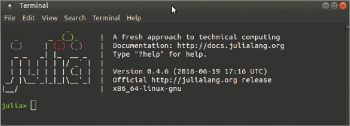
On successful installation, type ‘Julia’ at the terminal to start Julia. The welcome screen of Julia is shown in Figure 1.

Julia execution modes
Julia can be executed in three different ways as illustrated in Figure 2.
- Command line execution: To work in this mode, just download Julia as mentioned above and start working at the terminal by typing julia.
- Using the Integrated Development Environment Juno: To work in this mode, first the Julia command line needs to be downloaded. If Atom is not installed in your system, then get it from https://atom.io/. After the successful installation of Atom, navigate to the Settings::Install panel (press Ctrl to open Settings). Enter uber – juno and install the same.
- Using JuliaBox.com. No installation is required for this mode. You can visit this URL and start interacting with Julia.
The features of Julia
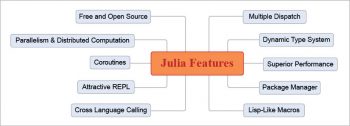
The significant features of Julia are illustrated in Figure 3. This language has the ability to define function behaviour across many combinations of parameter types. This feature is known as Multiple Dispatch. Availability of an in-built package manager, attractive REPL, the ability to execute code in a parallel and distributed environment, and optimal code generation are the other noteworthy features of Julia.
Julia REPL
Julia provides an attractive REPL (Read – Evaluate – Print – Loop), which facilitates the execution of Julia expressions. The expressions are evaluated immediately and the results are printed.
julia> 5 + 3
8
If you enter a ‘?’ in the REPL, it will switch to the HELP mode. In this mode, you may enter keywords and search for information on them. In the HELP mode, the prompt changes to yellow.
help?> peakflops()
  ..  peakflops(n; parallel=false)
‘peakflops’ computes the peak flop rate of the computer by using double precision :func:`Base.LinAlg.BLAS.gemm!`. By default, if no arguments are specified, it multiplies a matrix of size ‘n x n’, where ‘n = 2000’. If the underlying BLAS is using multiple threads, higher flop rates are realised. The number of BLAS threads can be set with blas_set_num_threads(n).
If the keyword argument ‘parallel’ is set to ‘true’, ‘peakflops’ is run in parallel on all the worker processors. The flop rate of the entire parallel computer is returned. When running in parallel, only one BLAS thread is used. The argument ‘n’ still refers to the size of the problem that is solved on each processor.
The code above provides helpful information regarding the peakflops().
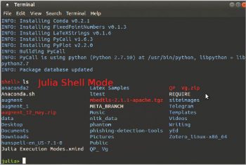
To enter into shell mode, press ‘;’. From the shell mode, you can execute shell commands, as shown in Figure 4. In the shell mode, the prompt changes to red.
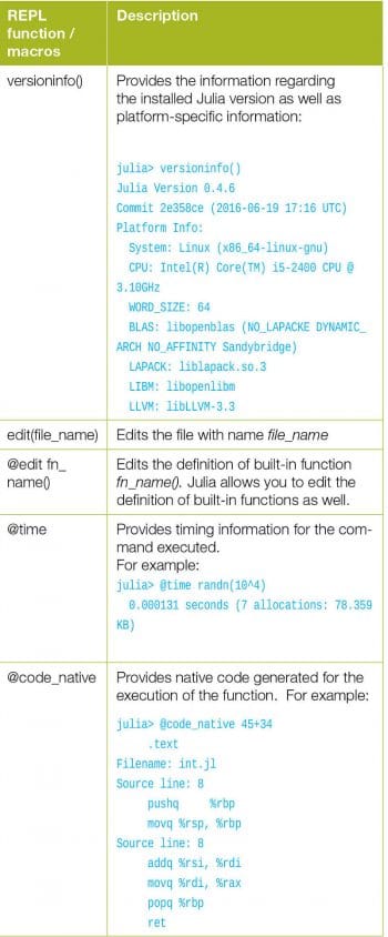
The REPL provides many more functions. A few popular functions and their descriptions are provided in Table 1.
The power of Julia
An interesting introduction to Julia by one of its co-creators, Viral Shaw, is available at https://www.youtube.com/watch?v=6fioFiKMXFk. The illustration provided in this video enables us to understand and appreciate the power of Julia.
As stated earlier, Julia code runs very fast. Let’s prove that with a simple but powerful example:
function test(n::Array)
  sum = 0.0
  for i = 1:length(n)
    sum+=n[i]
  end
  println(sum)
end

num = randn(10^7)
@time test(num)
The code above has a simple function to navigate through an array and find the sum of elements. The real power of Julia lies in the scalability. The code has a statement to generate 10 to the power of seven (10 million) random numbers (with normal distribution).
num = randn(10^7)
The 10 to the power of seven elements array is supplied as an input to the function. Julia is capable of looping through the 10 million elements array and finding the sum in 0.016 seconds.
The output is:
1332.9215017279294
0.016124 seconds
The code was modified to loop through 10 to the power of 8 (100 million) elements, and Julia was able to give the result in 0.120297 seconds.
8247.19158291053
0.120297 seconds (2.03 k allocations: 102.361 KB)
Note that the successive execution of code is comparatively faster than the first time execution. This is due to the JIT (Just in Time) compilation adopted by Julia.
Let’s take a look at another example that involves the multiplication of two matrices of size 1000×1000 and its timing values.
a = randn(1000,1000)
b = randn(1000,1000)
@time a*b
The output is:
0.041690 seconds (9 allocations: 7.630 MB, 5.00% gc time)
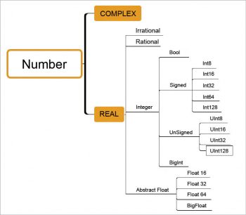
Julia focuses on numeric processing. It has an extensive hierarchy of types for handling numbers (as shown in Figure 5).
Type neutral function definition
Julia facilitates the defining of generic functions. Let’s consider the following example.
Define a generic function:
julia> f(x) = 4x^3+3x^2+8
f (generic function with 1 method)
Call f(x) with an integer value:
julia> f(5)
583
Call f(x) with a float value:
julia> f(25.67)
69645.719752
Note that we didn’t make any modification to the function definition when calling with a different data type. This generic function definition is a very important feature of Julia.
Cross-language calls
Julia has the option to call functions from languages such as Python, C, Fortran, etc. This facilitates seamless integration between components written in different languages.
For example, to call Python functions from Julia, type:
using PyCall
@pyimport math
math.sin(math.pi / 4) - sin(pi / 4)  # returns 0.0
@pyimport is used to import the sub-modules of Python.
Julia packages
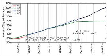
Another interesting feature of Julia is the extensibility similar to what we have in languages like Python. As of July 3, 2016, the official repository has 1035 packages. The evolution of the package ecosystem (http://pkg.julialang.org/pulse.html) is illustrated in Figure 6.
Primarily, packages enable us to extend the functionality of the core Julia engine. The areas covered by the packages are really diverse in nature. There are packages available for mathematical operations, machine learning, GUI, etc.
To add a package, enter the following command at the Julia prompt:
Pkg.add(“ package name”)
Pkg.add(“PyPlot”)
To use the package, the using keyword is employed:
using PyPlot
Plotting with Julia
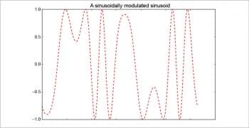
Julia facilitates plotting as well. A sample code is shown below:
using PyPlot
x = linspace(0,2*pi,1000); y = sin(3*x + 4*cos(2*x));
plot(x, y, color=”red”, linewidth=2.0, linestyle=”--”)
title(“A sinusoidally modulated sinusoid”)
The output plot of the above code is shown in Figure 7. (The successful execution of this code requires Python and MatPlotLib availability in the system.)
Julia is certainly a promising programming language, and its use is on the rise among scholars and data scientists. In the years to come Julia will evolve further; so try and get familiar with its ecosystem. The Julia home page has plenty of resources in the form of PDFs, video lectures, live notebooks, books, blogs, etc, which makes the process of getting insights into the Julia development process simple, efficient and enjoyable. Computing with Julia can really be awesome. Give it a try.


