Scilab (http://www.scilab.org) is open source software for numerical computation with a syntax similar to MathWorks MATLAB. Scilab has very good plotting capabilities, but some plot types are not available as primitives or functions. So, its necessary to write some code to obtain them. Note that the keywords of Scilab are categorised as primitives, commands, variables, functions and xcos functions. These words will be used only in reference to the keywords. To avoid any confusion, the word variable in the sense of a physical quantity (or chemical, graphical …) will be replaced by the word parameter. In this article, seven new (or almost new) plot types are covered with some practical applications, all made with Scilab 5.5.1 under Linux Mint 17 Xfce. Because the full code for each example is too long for a printed article, it’s freely (as in freedom and in beer) available at https://github.com/astonfe/scilab
Area plot
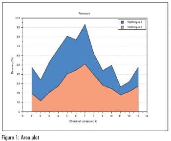
In this first example, we need to graphically compare two series of experimental data. These two columns are the per cent recoveries of 13 chemical compounds extracted from environmental samples using two different techniques. We can plot the data with the function bar or with an area plot (or a wide range of other tools, but this is only an example), which requires a bit of coding. This is easy to do because each area can be defined by a combination of the function plot and the primitive xfpoly, which is a filled polygon with the base at y=0 (see the parameter base).
Bar plot 3D
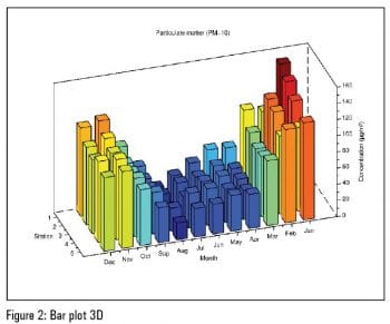
This example is about analysing particulate matter in urban air. The parameters are three: concentration, month of the year and monitoring station. Each measure is a point in this three-dimensional space. The function hist3d can be an option, but this plot type is not very nice (its a bit ugly). Even in this case, some coding is required. The plot is built by scanning the data matrix with two nested loops. Each parallelepiped has a square base with the side w equal to 0.8 and the height z equal to the concentration. The parameter col is used to scale the colours by aligning the data and the colour map. Note that in Scilab, it is possible to use special characters directly in SciNotes, the built-in editor. SciNotes is a powerful text editor and it also has interesting LaTeX capabilities (some examples will be shown in the following sections about impulse and ternary plots). At present, its not possible to automatically align the x axis and y axis labels to the respective axis orientation, since x_label.font_angle and y_label.font_angle are not specified. The code is partially based on the Scilab code written by Alex Carneiro (see http://usingscilab.blogspot.it/2012/09/plot3d2-creating-cube.html).
Impulse plot
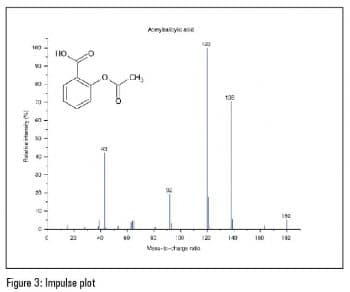
This plot type can be used to plot a mass spectrum. In this example, the acetylsalicylic acid (2-acetoxybenzoic acid) mass spectrum is considered. The peak data are taken from http://sdbs.db.aist.go.jp/sdbs/cgi-bin/direct_frame_top.cgi and then organised in four columns. The first two columns are the spectrum coordinates and the second two are the fragments coordinates, on which the numerical labels are put. With the LaTeX command includegraphics and the primitive xstring, its also possible to add an image of the molecular structure (via the parameter g). In xstring (5,65,$+g+$), first the coordinates are written about the position of g on the plot and then g is inserted between two $. That is how LaTeX can be used with Scilab. If the impulses are plotted horizontally, the result can be adapted to something similar to a Gantt chart.
Radar plot
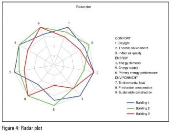
The radar or spider plot can be used to represent one or more data series in a form similar to a polar plot. A practical example is given by the radar plot widely used by Active House (http://www.activehouse.info) for displaying nine parameters about comfort, energy and the environment in the design of a building and in the finished building. Basically, the structure of this plot is built on a bi-dimensional grid via the function meshgrid. There are also a lot of settings with the functions gca, gce and with the primitive get. The legend is divided into two parts: the first is written with the primitive xstring and the second with the function legends. Due to the large legend, the plot has shifted a bit on the left side. The code is adapted to Scilab from the MATLAB code written by Cheng Li (see http://www.mathworks.com/matlabcentral/fileexchange/30305-spider-rader–chart-for-multi-data).
Ribbon plot
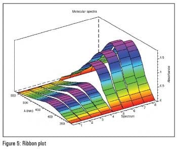
Now lets consider one absorbance spectrum measured from 350 nm to 550 nm (steps of 10 nm each) and at eight different times. So the data table is composed of eight columns. The most important thing about this plot type is how to use the function cat within the function surf. The result is that each z value (each column) is duplicated because, in this case, it must be a real matrix defining the surface height.
Ternary plot
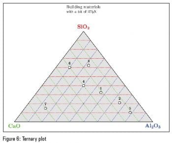
A ternary plot is used in physical chemistry, petrology, mineralogy, metallurgy and other physical sciences to show the compositions of systems composed of three species. Its also used in population genetics and in game theory [see http://en.wikipedia.org/wiki/Ternary_plot]. In this example, the compositions of certain building materials are shown as in a similar example in the book Inorganic Industrial Chemistry by Büchner, Schliebs, Winter, Büchel (see References at the end of the article). The original data are easily converted to the triangular coordinates using the parameters xx and yy. The coloured grids are built using a particular loop containing a combination of the primitives xset and xpoly. All the labels are written with a LaTeX notation. The code is partially based on the Gnuplot code written by Atsushi Noda (http://staff.aist.go.jp/a.noda/programs/ternary/ternary-en.html).
Time plot
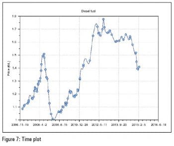
Sometimes, its necessary to observe how a parameter varies over time. The plot has the parameter on the y axis and the time on the x axis. In this example, the data is organised in four columns: year, month, day and price of the diesel fuel. The function datenum is first used to convert the original data (the first three columns) to the x coordinates and then the function datevec is used to create the labels on the x axis. Last, a fast cubic spline is used for connecting the points.
If you are in need of a plot type thats not available in Scilab, by default, you can write it with some lines of code. The code necessary for the calculations is relatively short and most of it (and perhaps, the most boring part) is dedicated to the colour and label settings. There are also other plot types that can be reproduced in Scilab fairly easily.
References
[1] http://usingscilab.blogspot.it/2012/09/plot3d2-creating-cube.html, last visited on 27/03/2015.
[2] http://sdbs.db.aist.go.jp/sdbs/cgi-bin/direct_frame_top.cgi, last visited on 27/03/2015.
[3] http://en.wikipedia.org/wiki/Ternary_plot, last visited on 27/03/2015.
[4] Büchner, Schliebs, Winter, Büchel, Chimica inorganica industriale (Inorganic industrial chemistry), Piccin, Padua, 1996.
[5] http://staff.aist.go.jp/a.noda/programs/ternary/ternary-en.html, last visited on 27/03/2015.
[6] http://www.mathworks.com/matlabcentral/fileexchange/30305-spider-rader–chart-for-multi-data, last visited on 27/03/2015.


