SageMath: A Second Glance at Cybersecurity

The eighth article in the series on SageMath explores a classical encryption scheme called the Rail Fence cipher and introduces the concept of symmetric-key encryption.

In the previous article in this SageMath series (published in the November 2024 issue of OSFY), we began exploring cybersecurity and introduced classical encryption techniques, setting a foundation for further discussion. In this article, we delve into a classical encryption scheme known as the Rail Fence cipher. Unlike the Caesar and Vigenère ciphers we covered earlier—both of which are substitution ciphers that replace each plaintext letter with another to create the ciphertext—the Rail Fence cipher is a transposition cipher. Here, letters in the plaintext are rearranged rather than substituted, producing a scrambled version of the plaintext to form the ciphertext. Notice that any terms introduced without explanation here were discussed in the previous article.

Before proceeding further, we need to focus on two additional aspects as we progress in this series, beyond discussing SageMath code. First, we need to set up effective tools for working with SageMath. Second, we should explore the historical context of our topic: cybersecurity and cryptography.

Let us start by addressing a tool-related issue. So far, we have been using an online platform called CoCalc, a web-based tool well-suited for running SageMath programs. However, CoCalc operates on a freemium model, requiring payment for certain features. While I am not an ardent advocate of exclusively using free and open source software, I initially recommended CoCalc for its accessibility. Since SageMath has a steep learning curve, I thought it would be beneficial for those new to it to quickly access an online tool rather than navigate the challenges of installing it on their preferred operating system. However, it is now time to explore alternative tools and options beyond CoCalc.

Installing and using SageMath on your computer

Let us start by installing SageMath on your computer. The installation process can vary depending on the version of SageMath you choose and the operating system you use. As mentioned earlier in this series, the latest version of SageMath supported by CoCalc is version 10.4. Installing this version manually on your computer can be a lengthy process, but you can find detailed instructions on the SageMath website.

If you are open to using a slightly older version, the process becomes much easier. For instance, installing SageMath on Ubuntu is straightforward. Simply open the GNOME Software application (commonly referred to as Ubuntu Software or Ubuntu Software Center), search for ‘SageMath’, and click the Install button. Enter your root password when prompted, and the installation will be completed in no time. Other Linux distributions and operating systems likely offer a similarly simple process. However, note that this method typically installs version 9.0 of SageMath.

I have been using version 9.0 for some time and find it perfectly capable. Personally, I prefer sticking with stable software rather than frequently updating just to gain a feature I may never use. Ultimately, the choice of version and installation method is yours, based on your needs.

Assuming you have a reasonably recent version of SageMath installed, let us explore how to use it locally. SageMath is like a curious and resourceful individual—it adopts the best tools it encounters. For example, SageMath integrates the IPython shell into its interactive environment. This enhanced IPython-based interface offers powerful features like magic commands (%time, %timeit, %run, etc), tab completion, and syntax highlighting.

To experience this, open a terminal, type the command sage, and press the Enter button. This will launch the SageMath interactive shell (Figure 1).

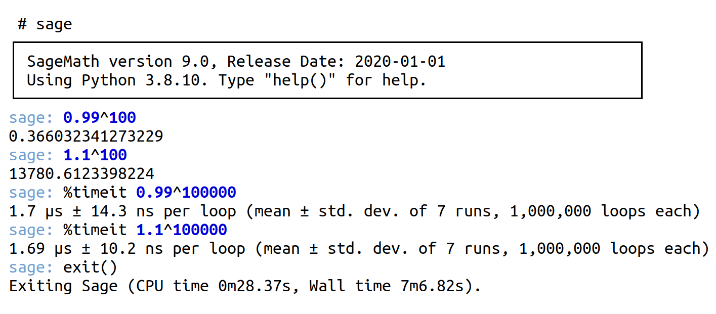
As shown in Figure 1, I am using SageMath version 9.0 along with Python 3.8.10. I subscribe to the philosophy, “If it ain’t broke, don’t fix it.” I only update software when it directly impacts my work, rather than simply because a new version is available and I have received an update notification.

In the example commands shown in Figure 1, the first two lines demonstrate execution of basic mathematical operations and display the results. The third and fourth lines illustrate how to measure the execution time of calculations using the %timeit magic command. This command executes the expressions ‘0.99^100000’ and ‘1.1^100000’ multiple times, calculating an average execution time. Such an approach provides a more reliable performance assessment, particularly for operations that execute very quickly. From Figure 1, it is evident that SageMath is both fast and powerful, making it an invaluable computational tool. Finally, the exit( ) command is used to exit the shell, functioning similarly to its usage in IPython.

Now, let us learn how to execute saved SageMath programs. Consider the single-line SageMath program named test.sage, as shown below.

Note that this is essentially Python code in disguise, as SageMath is built on Python syntax. To run the program test.sage, execute the following command in a terminal:

You will now see the text “This is a very simple SageMath code” printed on the terminal. But what happened to the .sagews extension that we used for all the programs discussed earlier in this series? This extension is typically associated with SageMath worksheets, commonly used in platforms like CoCalc and JupyterLab. However, for standard SageMath scripts, the .sage extension is more appropriate.

A brief history of the beginnings of modern cryptography

Before delving into more complex codes, let me take you through a brief history to understand the evolution of cybersecurity and cryptography.

While the two World Wars brought immense human suffering, they also drove significant advancements in science and technology, resulting in inventions like nuclear energy, digital computers, airplanes, submarines, and more. Cryptography was one such field that underwent a revolutionary transformation during this period.

In World War I, substitution ciphers like the Playfair cipher were commonly used. A pivotal moment in the war occurred when British intelligence intercepted and deciphered the Zimmermann Telegram—a secret communication from the German ambassador to Mexico. This breakthrough played a significant role in the United States entering the war.

World War II saw the Germans rely heavily on the Enigma machine, an electromechanical device they believed to be unbreakable. However, much like the French during the Franco-Prussian War of 1870, the Germans underestimated their adversaries. British intelligence successfully cracked the Enigma’s encryption scheme, marking a turning point in the Allies’ victory in World War II.

This monumental achievement was led by Alan Turing, one of the most influential figures in computer science. His work not only contributed to the Allies’ success but also laid the foundation for modern computing and cryptography. The Hollywood film ‘The Imitation Game’ vividly portrays the cracking of the Enigma codes and the tragic life of this extraordinary individual.

World War II also accelerated the development of digital computers, which paved the way for more sophisticated encryption schemes and heralded the beginning of modern cryptography.

Transposition ciphers

Let us now explore another classical encryption scheme, the Rail Fence cipher, before moving onto modern encryption techniques. The Rail Fence cipher is a transposition cipher that rearranges the positions of characters without altering the characters themselves. For example, the word ‘listen’ can be rearranged to form ‘silent’.

To understand the Rail Fence cipher, let us walk through a simple example. In a simplified version of this cipher, the plaintext is written column by column into a grid and then read row by row to generate the ciphertext. The number of rows in the grid, known as the number of rails, is determined by the encryption scheme designer. The example below demonstrates how the plaintext ‘CONSIDERABLE’ is encrypted using three rails.

Upon reading the plaintext row by row, we obtain the ciphertext ‘CSEBOIRLNDAE’. Decryption follows a similar process: the ciphertext is written row by row, and then read column by column to reconstruct the original plaintext.

Now, let us consider the program railfence.sage, which implements this simplified version of the rail fence encryption scheme. To simplify further, we assume that only uppercase letters are used, and no whitespaces are present. The code below performs the encryption process in the program railfence.sage (line numbers are included for clarity).

Now, let us go through the code line by line to understand how it works. Line 1 defines a function named rail_fence_encrypt. It takes two arguments: plaintext, which contains the text to be encrypted and num_rails, which specifies the number of rows (rails) to use in the Rail Fence cipher. Line 2 creates a list rails with num_rails empty strings, one for each rail. For example, if num_rails = 3, then rails will be [‘’, ‘’, ‘’]. These strings will store the characters assigned to each rail during encryption. Line 3 iterates over each character in the plaintext. The enumerate( ) function provides the index of the character in the plaintext and the character itself. Line 4 distributes characters to rails. The result of ‘i % num_rails’ cycles through 0, 1, 2, …, (num_rails-1), ensuring characters are distributed cyclically across the rails. Line 5 joins all the strings in the list rails into a single string, ciphertext. Line 6 returns the encrypted text (ciphertext) as the output of the function.

The code below performs the decryption process in the program railfence.sage (line numbers are included for clarity):

Now, let us go through the code line by line to understand how it works. Line 7 defines the rail_fence_decrypt function. It takes two arguments: ciphertext, which contains the encrypted message and num_rails, which specifies the number of rows (rails) used during encryption. Line 8 determines how many characters belong to each rail. Line 9 creates an empty list rails to store substrings of ciphertext corresponding to each rail. Line 10 sets the index pointer idx to 0. This will track the current position in the ciphertext while splitting it into rails. Line 11 loops through each rail’s length in rail_lengths. Line 12 extracts a substring from the ciphertext starting at idx with a length equal to length and appends the substring to the list rails. Line 13 moves the index pointer idx forward by the length of the current rail, preparing for the next slice. Line 14 creates an empty string plaintext to hold the reconstructed message. Line 15 iterates through the ciphertext, one character at a time, based on its length. Line 16 calculates the index of the rail (rail_idx) from which the next character should be taken. The modulus operator (%) is used to cycle through the rails. Line 17 appends the first character ([0]) from the current rail (rails[rail_idx]) to plaintext. Line 18 removes the first character from the current rail after it is added to plaintext. Line 19 returns the fully reconstructed plaintext as the output of the function.

The code below performs the testing process in the program railfence.sage (line numbers are included for clarity):

Now, let us try to understand how the testing works. Line 20 assigns the plaintext message ‘OPENSOURCEFORYOU’ to the variable plaintext. This message will be encrypted using the rail fence cipher. Line 21 sets the number of rails (rows) to 3. This determines how the plaintext will be arranged during the encryption process. Line 22 calls the function rail_fence_encrypt, passing plaintext and num_rails as arguments. The function encrypts the plaintext using the Rail Fence cipher and assigns the resulting ciphertext to the variable ciphertext. Line 23 calls the function rail_fence_decrypt, passing ciphertext and num_rails as arguments. The function decrypts the ciphertext using the Rail Fence cipher and assigns the resulting plaintext to the variable decrypted_text. Lines 24 to 26 display the plaintext, its encrypted ciphertext, and the decrypted ciphertext, confirming the successful encryption and decryption process.

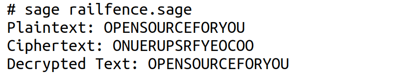
The SageMath program railfence.sage can be executed by running the command sage railfence.sage in a terminal. Figure 2 shows the execution and output of the SageMath program railfence.sage. To verify the program’s functionality, replace Line 20 with the following line of code: plaintext = “CONSIDERABLE”. Executing this modified program should yield the ciphertext ‘CSEBOIRLNDAE’, as expected from our earlier example. Next, in the original code, replace Line 21 with the following line of code: ‘num_rails = 4’. Running this modified program will produce the ciphertext ‘OSCRPOEYEUFONROU’, confirming that the encryption result varies with the number of rails. With this discussion, we have covered some key classical encryption techniques. It is now time to advance to modern cryptographic methods.

Introduction to symmetric-key cryptography

Symmetric-key cryptography is a cornerstone of modern cryptography, providing efficient and secure methods for protecting data in applications such as secure communications, financial transactions, and data storage. This type of encryption employs a single key for both encrypting and decrypting data. The security of this method hinges on the secrecy of the key, which must be shared confidentially between the sender and receiver.

Common symmetric-key algorithms include the Advanced Encryption Standard (AES) and the Data Encryption Standard (DES). While these algorithms are efficient and fast, the primary challenge in symmetric-key cryptography lies in the secure distribution and management of the secret key between the involved parties.

To implement many of the cryptographic functions discussed in this series, we will need to install PyCryptodome, a Python package that provides implementations for a variety of cryptographic algorithms. SageMath, a powerful mathematical software, can leverage the functionalities offered by PyCryptodome. To install PyCryptodome, simply execute the following command in your terminal: pip install pycryptodome. With PyCryptodome installed, you gain access to a comprehensive suite of cryptographic tools, including symmetric-key algorithms such as AES and DES, public-key algorithms like RSA, and hash functions like SHA-3 and BLAKE2.

DES (Data Encryption Standard) is a symmetric-key encryption algorithm used to secure data. It encrypts data by using a fixed-size key to transform the original data into ciphertext and can decrypt it back to the original using the same key. While DES was widely used in the past, it is now considered outdated and less secure due to advances in computational power. However, as the first example, we will discuss the implementation of DES as illustrated in the SageMath program named des.sage shown below (line numbers are included for clarity).

Now, let us go through the code line by line to understand how it works. Line 1 imports the DES cipher class from the module Crypto.Cipher of the PyCryptodome library, which provides the implementation for the DES encryption algorithm. Line 2 imports two functions, pad and unpad, from the module Crypto.Util.Padding. These functions are used to handle padding for data, which ensures the input is a multiple of the DES block size (8 bytes). Line 3 defines a secret key for the DES algorithm. The b before the string indicates it is a byte string, which is required for cryptographic operations. In this case, the key is “RAINBOWS”, an 8-character string, which is the exact length required for DES. Line 4 creates a new DES cipher object with the specified key and sets the encryption mode to ECB (Electronic Codebook), one of the simplest modes for block ciphers, where each block is independently encrypted. Line 5 defines the plaintext message to be encrypted: “HAPPINESSISABUTTERFLY”. Since DES works on fixed block sizes, the plaintext may need padding. Line 6 prints the original plaintext message to the console for reference. Line 7 encodes the plaintext (converts it into bytes) and then applies padding using the pad function. The padding ensures that the byte length of the plaintext is a multiple of the DES block size (8 bytes). Line 8 encrypts the padded plaintext using the DES cipher and stores the resulting ciphertext in the variable ciphertext. Line 9 prints the ciphertext in hexadecimal format for better readability, as the output of the encryption is binary data. Line 10 decrypts the ciphertext using the same DES cipher and stores the result in decrypted_padded. The result is still padded to align with the block size. In Line 11, the decrypted message is passed through the function unpad to remove the padding, and is then decoded (converted back from bytes to a string) to retrieve the original message. Line 12 prints the decrypted message, which should match the original plaintext, confirming that the encryption and decryption processes worked correctly.

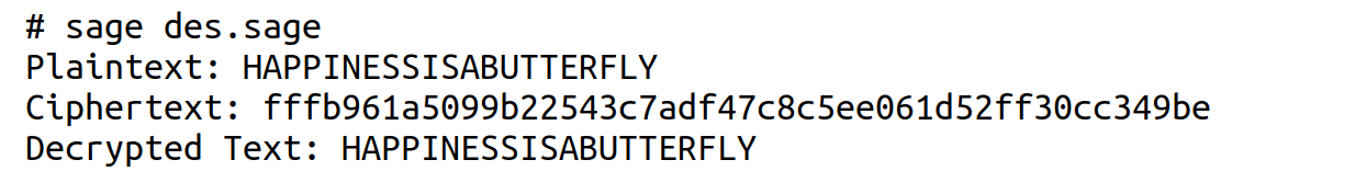
Upon execution, the program des.sage generates the output shown in Figure 3. But how does DES work? We will explore this in detail in the next article in this series.

As we wrap up this article, we have broadened our understanding of key cybersecurity terminology. We explored Rail Fence encryption and introduced the concept of symmetric-key encryption. However, there is still much to explore in the realm of symmetric-key cryptography. In the next article, we will continue our discussion by exploring the working of the Data Encryption Standard (DES) and other key developments in this area.