


If you do not consider yourself a Calc or Excel expert but must do your taxes in a spreadsheet, then these cool tricks can help you a great deal.
The financial year ended in March and everyone with taxable income must file IT returns by July this year. I opened a new bank account last year and it came with a new demat (share-trading) account. Rather than just shovel numerous lists of transactions from my bank and demat accounts to my tax consultant, I decided to put all that data in one spreadsheet before sending it to him. My experience with spreadsheets ended with Lotus 1-2-3 in the 90s so working with Calc threw several challenges. Here is how I addressed them.
IF function — for conditional formulae
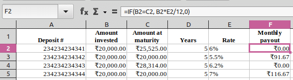
Some fixed deposits make interest payments at a regular interval (monthly, quarterly, half-yearly or yearly) while others pay cumulative interest only at maturity. How do I make a column for monthly interest payments for a list that contains both types of deposits? If the amount paid back by a fixed deposit at maturity is the same as the amount invested at the beginning, then it would have paid interest at regular intervals. If the amount paid back at maturity is much greater than the amount invested at the beginning, then obviously, it must be a cumulative fixed deposit.
In Figure 1, the F column contains formulae with the IF function. The monthly payout is calculated only if the pay-in and payout are the same.
| Deposit # | Amount invested (Rs) |
Amount at maturity (Rs) | Number of years |
Rate of interest |
Monthly payout |
| 234234234341 | 20000 | 25525 | 5 | 6% | =IF(B2=C2, B2*E2/12,0) |
| 234234234342 | 20000 | 20000 | 5 | 5.5% | =IF(B3=C3, B3*E3/12,0) |
| 234234234343 | 20000 | 28314 | 5 | 6.2% | =IF(B4=C4, B4*E4/12,0) |
| 234234234344 | 20000 | 20000 | 5 | 7% | =IF(B5=C5, B5*E5/12,0) |
SUMIF function — for conditional totals
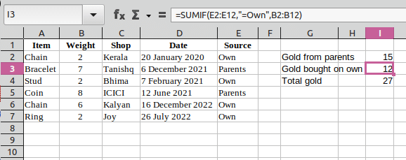
I have listed my gold ornaments in a spreadsheet. I have bought most of the gold but some came from my parents. Because share-trading platforms routinely demand to know my net worth, I need to calculate how much of the gold is my own and how much is not.
In Figure 2, the E column shows the source of the gold ornament and the B column gives its weight. Using the SUMIF function, I can add the weights in the B column if the corresponding values in the E column equal a particular type of source. This can be done using the search criterion as either “=Own” or “=Parents”.
| Item | Weight | Shop | Date | Source | |||
| Chain | 2gm | Kerala | 20 January 2020 | Own | |||
| Bracelet | 7gm | Tanishq | 6 December 2021 | Parents | Gold from parents | =SUMIF(E2:E12,”=Parents”,B2:B12) | |
| Stud | 2gm | Bhima | 7 February 2021 | Own | Gold bought on own | =SUMIF(E2:E12,”=Own”,B2:B12) | |
| Coin | 8gm | ICICI | 12 June 2021 | Parents | Total gold | =SUM(B2:B12) | |
| Chain | 6gm | Kalyan | 16 December 2022 | Own | |||
| Ring | 2gm | Joy | 26 July 2022 | Own | |||
VLOOKUP function — for values from a lookup table
I have a list of stocks in my portfolio. Can Excel or Calc show me their worth based on the LTPs (last traded prices)? There are some web services that provide the latest stock quotes but these are all paid services. The National Stock Exchange (NSE) does publish the quotes on its website. I cannot write a shell script to download it because they use a dynamic link specifically to foil script writers like me.
The only choice is to manually download the market data from the NSE site. From the site menu, choose MARKET DATA » Equity & SME Market » NIFTY TOTAL MARKET » Download(.csv). Open the CSV (comma separated values) file and copy the data to a new worksheet in your Calc file. There will be over 750 rows to copy. (From the first cell, use Ctrl+Shift+Right and Ctrl+Shift+Down keys to select the whole data.)
Name the worksheet as NSE_MARKET_DATA. For each stock, the trading symbol (code or ID) will be in the A column. The LTP will be in the F (sixth) column.
In other worksheets, I use a VLOOKUP function wherever I want to display data from the NSE_MARKET_DATA worksheet. (The NSE_MARKET_DATA worksheet is the lookup table.) The first parameter of the function is for the value that I want to look up. The second parameter is the target range in the worksheet containing the lookup table (market data). The third parameter is the column number in the target range that contains the required data corresponding to the looked-up value. The last parameter is set to FALSE or 0 as the market data is not expected to be sorted.
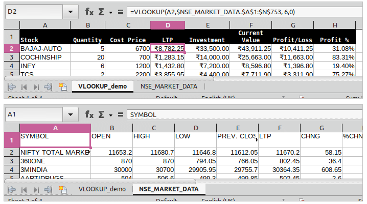
For example, look at this formula in the second row of Figure 3:
=VLOOKUP(A2,$NSE_MARKET_DATA.$A$1:$N$753, 6,0)
The lookup table is locked-in using dollar characters ($NSE_MARKET_DATA.$A$1:$N$753). The A column contains the stock ID. After I specify the formula as shown above, the LTP price of the stock will be copied from the lookup table in the NSE_MARKET_DATA worksheet and displayed in the current worksheet.
Figure 3 shows the main worksheet; the stock symbol is in the A2 cell. The VLOOKUP formula is in the D2 cell. In the worksheet containing the lookup table, the value being looked up is in the first column and the value being copied is in the sixth column.
INDEX and COUNT functions — for the last cell in a column
Net banking websites provide downloadable spreadsheet files that contain the list of transactions in your account. The last cell in the statement contains your current balance. However, in a financial year, the list of transactions grows and the location of the last cell moves. How can you find the last cell in a column using a formula?
The trick is to use both INDEX and COUNT functions. The INDEX function can use row and column coordinates to obtain a value from a range of cells. The COUNT function can count the number of cells that are not empty.
Using the two functions together, I came to this formula:
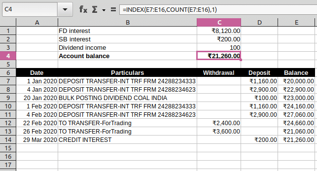
=INDEX(E7:E16,COUNT(E7:E16),1)
To limit the size of the screenshot, I used only a few rows in the example (E7:E16) including blank ones. A typical list of transactions will have hundreds of rows so a much larger range will be required.
Figure 4 shows the function COUNT(E7:E16) returns 8 as the number of rows in the list of transactions. Thus, the INDEX function just needs to go to the 8th cell down from E7 to find the final account balance.
Convert text to columns
If you download your list of transactions from your net banking site as a spreadsheet or CSV, not all cell values may be appropriately converted. It is likely that numbers and dates are all prefixed with a single quote (“ ‘ “) to prevent their values from being converted to illogical values. For example, to prevent a long number 23423234234234 from being converted as an exponential value 234232E+12 (which loses precision as it gets rounded off), it may be specified as text as ‘23423234234234.
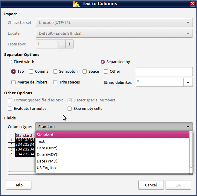
When cell values contain text rather than numbers and dates, you cannot apply formulae on them from other cells. Rather than leave them as they are, you may need to study each set of cells first and convert appropriately. There is a Text to Columns… option in the Data menu of Calc but it is not very intuitive. It works only on one column at a time. That is, you cannot convert multiple columns at a time. The correct procedure is:
- Select the cells (in a column) that need to be converted to numbers or dates.
- Select Data » Text to Columns… from the Calc main menu.
- In the Text to Columns dialog that opens up, click on the cells preview in the Fields section.
- Choose an option in the Column type list, which will now be populated with appropriate target value types for the cells that you have clicked and selected in the previous step.
The bottomline
People who use Excel or Calc everyday may find these functions as nothing out of the ordinary. For someone who has used spreadsheet programs only to sort lists or do simple totals, these conditional functions can seem mind-blowing.


