


The third article in the ongoing series on FOSS security tools introduces the Scapy packet program and library.
Scapy is a packet manipulation library written in Python that can also be used interactively. You can create and decode packets for a number of protocols, and also store them in a packet capture (pcap) file. It can perform scans, probes, network discovery, traceroutes, attacks, and has many features of tools like Nmap, tcpdump, Wireshark, etc. Released under the GNU GPL 2.0 licence, its source code is available on GitHub. It requires at least Python 3.7 and has cross-platform support.
Installation
You can install Scapy on Ubuntu using the following command:
$ sudo apt install python3-scapy python3-pyx python3-geoip python3-cartopy
The pyx package is useful for generating PostScript graphics output. The python3-geoip and python3-cartopy packages can produce traceroute and visualisation maps. The version of Python3 used for this article is 3.10.12 from Ubuntu 22.04.4 LTS system as shown below:
$ python3 --version
Python 3.10.12
You can invoke the ‘scapy’ tool directly from the command line, but you will need to use it with the ‘sudo’ command for privileged commands.
$ sudo scapy
...
aSPY//YASa
apyyyyCY//////////YCa |
sY//////YSpcs scpCY//Pp | Welcome to Scapy
ayp ayyyyyyySCP//Pp syY//C | Version 2.4.4
AYAsAYYYYYYYY///Ps cY//S |
pCCCCY//p cSSps y//Y | https://github.com/secdev/scapy
SPPPP///a pP///AC//Y |
A//A cyP////C | Have fun!
p///Ac sC///a |
P////YCpc A//A | Craft packets like I craft my beer.
scccccp///pSP///p p//Y | -- Jean De Clerck
sY/////////y caa S//P |
cayCyayP//Ya pY/Ya
sY/PsY////YCc aC//Yp
sc sccaCY//PCypaapyCP//YSs
spCPY//////YPSps
ccaacs
using IPython 7.31.1

>>>
Configuration
The ‘lsc()’ command displays the default functions
in Scapy:
>>> lsc()

IPID_count : Identify IP id values classes in a list of packets
arpcachepoison : Poison target’s cache with (your MAC,victim’s IP) couple
arping : Send ARP who-has requests to determine which hosts are up
arpleak : Exploit ARP leak flaws, like NetBSD-SA2017-002.
bind_layers : Bind 2 layers on some specific fields’ values.
bridge_and_sniff : Forward traffic between interfaces if1 and if2, sniff and return
chexdump : Build a per byte hexadecimal representation
computeNIGroupAddr : Compute the NI group Address. Can take a FQDN as input parameter
The default routes can be viewed using ‘conf.route’ as shown below:
>>> conf.route
Network Netmask Gateway Iface Output IP Metric
0.0.0.0 0.0.0.0 192.168.111.1 wlp0s20f3 192.168.111.69 600
10.147.20.0 255.255.255.0 0.0.0.0 ztly546n2w 10.147.20.242 0
127.0.0.0 255.0.0.0 0.0.0.0 lo 127.0.0.1 1
169.254.0.0 255.255.0.0 0.0.0.0 virbr0 192.168.122.1 1000
172.17.0.0 255.255.0.0 0.0.0.0 docker0 172.17.0.1 0
192.168.111.0 255.255.255.0 0.0.0.0 wlp0s20f3 192.168.111.69 600
192.168.122.0 255.255.255.0 0.0.0.0 virbr0 192.168.122.1 0
The ‘dir()’ function is built-in and returns the names in the current scope as a list of strings:.
>>> dir()
[‘In’,
‘Out’,
‘_’,
‘_2’,
‘_20’,
‘_23’,
‘_26’,
‘_28’,
‘_32’,
‘_35’,
You can save the history of your commands in a session file using the ‘save_session()’ function as shown below:
>>> save_session(“trace.scapy”)
INFO: Use [trace.scapy] as session file
You can restore the session history from the file including the packets and data using the ‘load_session()’ function as follows:
>>> load_session(“trace.scapy”)
INFO: Loaded session [trace.scapy]
ICMP
Consider sending an Internet Control Message Protocol (ICMP) packet using the ‘send()’ function:
>>> send(IP(dst=”www.google.com”)/ICMP()).

Sent 1 packets.
The ‘sr()’ function is used for sending and receiving packets. The ‘sr1()’ function in module scapy.sendrecv is used for receiving only one packet. We can rerun the ICMP request as shown below:
>>> p = sr1(IP(dst=”www.google.com”)/ICMP())
Begin emission:
Finished sending 1 packets.
*
Received 1 packets, got 1 answers, remaining 0 packets
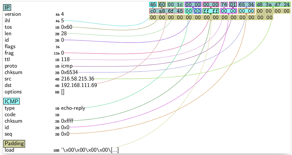
The returned packet field values can be listed as follows:
>>> p

<IP version=4 ihl=5 tos=0x60 len=28 id=0 flags= frag=0 ttl=118 proto=icmp chksum=0x64e1 src=216.58.215.36 dst=192.168.111.152 |<ICMP type=echo-reply code=0 chksum=0xffff id=0x0 seq=0x0 |<Padding load=’\x00\x00\x00\x00\x00\x00\x00\x00\x00\x00\x00\x00\x00\x00\x00\x00\x00\x00’ |>>>
A summary of the packet can be displayed using the ‘summary()’ function:
>>> p.summary()

‘IP / ICMP 216.58.215.36 > 192.168.111.69 echo-reply 0 / Padding’
A more detailed output of the returned packet can be viewed using the ‘show()’ method on the object as illustrated below:
>>> p.show()
###[ IP ]###
version= 4
ihl= 5
tos= 0x60
len= 28
id= 0
flags=
frag= 0
ttl= 118
proto= icmp
chksum= 0x64e1
src= 216.58.215.36
dst= 192.168.111.152
\options\
###[ ICMP ]###
type= echo-reply
code= 0
chksum= 0xffff
id= 0x0
seq= 0x0
###[ Padding ]###
load= ‘\x00\x00\x00\x00\x00\x00\x00\x00\x00\x00\x00\x00\x00\x00\x00\x00\x00\x00’
Graphical dump
Using the python3-pyx package, we can dump the packet contents into a PDF file as shown below:
>>> p.pdfdump(“/tmp/output.pdf”)
The PDF image of the output is shown in Figure 1. The other output options available are tabulated below.
|
Command |
Effect |
|
p.psdump() |
Output a PostScript diagram |
|
p.json() |
Return a JSON string representation of the packet |
|
p.show2() |
In addition to the show() command output, checksums are provided |
|
hexdump(p) |
A hexadecimal dump |
|
raw(p) |
The raw packet contents |
|
ls(p) |
The list of field values |
|
ls.sprintf() |
Use a format string with field values |
Traceroute
The ‘traceroute()’ function is in module scapy.layers.inet and can be used to trace a TCP route to a www.google.com server. For example:
>>> r = traceroute([“www.google.com”])
Begin emission:
Finished sending 30 packets.
******************************
Received 30 packets, got 30 answers, remaining 0 packets
216.58.215.36:tcp80
1 192.168.111.1 11
2 192.168.254.2 11
3 178.255.160.26 11
4 100.96.24.37 11
5 81.93.7.41 11
6 72.14.233.195 11
7 72.14.237.93 11
8 216.58.215.36 SA
9 216.58.215.36 SA
10 216.58.215.36 SA
11 216.58.215.36 SA
12 216.58.215.36 SA
13 216.58.215.36 SA
14 216.58.215.36 SA
15 216.58.215.36 SA
16 216.58.215.36 SA
17 216.58.215.36 SA
18 216.58.215.36 SA
19 216.58.215.36 SA
20 216.58.215.36 SA
21 216.58.215.36 SA
22 216.58.215.36 SA
23 216.58.215.36 SA
24 216.58.215.36 SA
25 216.58.215.36 SA
26 216.58.215.36 SA
27 216.58.215.36 SA
28 216.58.215.36 SA
29 216.58.215.36 SA
30 216.58.215.36 SA
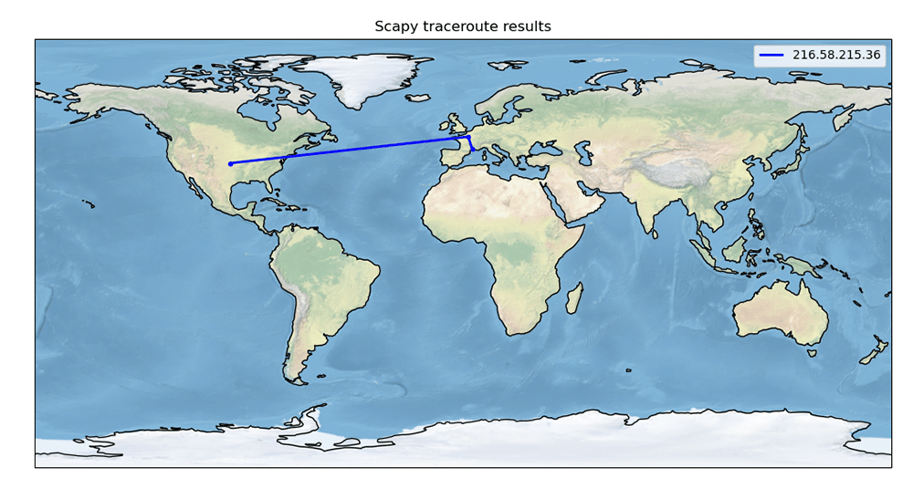
The GeoLite2-City.mmdb file provides an association mapping between cities and IP addresses. After downloading the same, you can import them to your configuration environment as follows:
>>> conf.geoip_city = “/home/user/GeoLite2-City.mmdb”
Using the ‘traceroute_map()’ function, a world map showing the traceroute path can be viewed:
>>> traceroute_map(“www.google.com”)
The world map with the trace route path is shown in Figure 2.
Sniff
The ‘sniff()’ function is used to capture packets in real-time. You will need to press ‘Ctrl+c’ to stop capturing the packets.
>>> sniff()
^C<Sniffed: TCP:51 UDP:8 ICMP:0 Other:0>
The captured packets can then be stored to a variable and the summary can be printed using the ‘nsummary()’ function as demonstrated below:
>>> s=_

>>> s.nsummary()
0000 Ether / IP / TCP 192.168.111.239:49152 > 192.168.111.81:59850 FPA / Raw
0001 Ether / IP / TCP 192.168.111.81:59850 > 192.168.111.239:49152 FA
0002 Ether / IP / TCP 192.168.111.81:59858 > 192.168.111.239:49152 S
0003 Ether / IP / TCP 192.168.111.239:49152 > 192.168.111.81:59850 A
You can also view a specific packet using the array subscript syntax:
>>> s[1]

<Ether dst=0c:91:60:5b:27:ec src=58:6c:25:ed:5d:d7 type=IPv4 |<IP version=4 ihl=5 tos=0x0 len=52 id=37178 flags=DF frag=0 ttl=64 proto=tcp chksum=0x48f8 src=192.168.111.81 dst=192.168.111.239 |<TCP sport=59850 dport=49152 seq=2775654087 ack=1975887132 dataofs=8 reserved=0 flags=FA window=501 chksum=0x60b8 urgptr=0 options=[(‘NOP’, None), (‘NOP’, None), (‘Timestamp’, (937481726, 627853))] |>>>
The ‘hexdump()’ function can output the hexadecimal values of the packets along with their ASCII text for reference.
>>> s.hexdump()
0000 01:10:59.618890 Ether / IP / TCP 192.168.111.239:49152 > 192.168.111.81:59850 FPA / Raw

0000 58 6C 25 ED 5D D7 0C 91 60 5B 27 EC 08 00 45 00 Xl%.]...`[‘...E.

0010 03 09 0F 2A 40 00 40 06 C8 33 C0 A8 6F EF C0 A8 ...*@.@..3..o...

0020 6F 51 C0 00 E9 CA 75 C5 A2 46 A5 71 1E C7 80 19 oQ....u..F.q....

0030 01 C5 94 64 00 00 01 01 08 0A 00 09 94 8D 37 E0 ...d..........7.

0040 D5 C6 72 76 69 63 65 49 64 3A 52 65 6E 64 65 72 ..rviceId:Render

0050 69 6E 67 43 6F 6E 74 72 6F 6C 3C 2F 73 65 72 76 ingControl</serv

0060 69 63 65 49 64 3E 0D 0A 3C 53 43 50 44 55 52 4C iceId>..<SCPDURL

0070 3E 2F 72 63 72 2E 78 6D 6C 3C 2F 53 43 50 44 55 >/rcr.xml</SCPDU

0080 52 4C 3E 0D 0A 3C 63 6F 6E 74 72 6F 6C 55 52 4C RL>..<controlURL
.If you have multiple network interfaces, you can explicitly specify the ‘iface’ attribute to capture the packets as demonstrated below:
>>> sniff(iface=”wlp0s20f3”, prn=lambda x: x.show())
###[ Ethernet ]###
dst= 33:33:00:00:00:fb
src= 72:71:d9:df:a3:b1
type= IPv6
###[ IPv6 ]###
version= 6
tc= 0
fl= 197632
plen= 262
nh= UDP
hlim= 255
src= fe80::840:4b79:ad35:c4dd
dst= ff02::fb
###[ UDP ]###
sport= mdns
dport= mdns
len= 262
chksum= 0xa5c7
PCAP
The capture packets can be written to a file using the ‘wrpcap()’ function.
>>> wrpcap(“output.cap”, s)
The packets can also be read from a file using the ‘rdpcap’ function as follows:
>>> data = rdpcap(“output.cap”)
Using the array subscription, you can get the detailed output for a specific packet:
>>> data[2]

<Ether dst=0c:91:60:5b:27:ec src=58:6c:25:ed:5d:d7 type=IPv4 |<IP version=4 ihl=5 tos=0x0 len=60 id=44535 flags=DF frag=0 ttl=64 proto=tcp chksum=0x2c33 src=192.168.111.81 dst=192.168.111.239 |<TCP sport=59858 dport=49152 seq=3260427060 ack=0 dataofs=10 reserved=0 flags=S window=64240 chksum=0x60c0 urgptr=0 options=[(‘MSS’, 1460), (‘SAckOK’, b’’), (‘Timestamp’, (937481726, 0)), (‘NOP’, None), (‘WScale’, 7)] |>>>
The ‘export_object()’ function allows you to export a packet to its base64 encoded representation:
>>> export_object(data[2])

b’eNprYEouTk4sqNTLSaxMLSrWyzHici3JSC3iKmTQDCpk1EiOT85PSU0u5kr NAzG4CpkiEhkYGHgOTUyIVj+8JiJH9fDa2MPTORhcGRhsDq09vN2BwYFNx/ww6EV+YFg8vD6wysPTzrcwHC4KUzbBKiX4dACpsO7D m9IAIoxMLGwHtrCwsTBZX54weGph/eB5BmZmdkLmSPY gMycxJLMPMNClrZC1qBCNqhTS0syc4q5XF1Sk zNzE3O4CtkjBIFKDc0NzS3NjAxMLfXMDC0NDY0KOVoLOYMKufz8/Ly9Sgq5k/QAox5N+Q==’
Build packets
The Scapy library allows you to construct packets from scratch. The ‘IP()’ function builds an IP packet with default values as demonstrated below:
>>> x=IP()
>>> x
<IP |>
>>> x.src
‘127.0.0.1’
>>> x.dst
‘127.0.0.1’
>>> x.ttl
64
>>> raw(x)
b’E\x00\x00\x14\x00\x01\x00\x00@\x00|\xe7\x7f\x0 0\x00\x01\x7f\x00\x00\x01’
You can stack protocols to build on the packet information. In the following example, we are adding a TCP and Ethernet packet to our IP packet layer:
>>> x/TCP()
<IP frag=0 proto=tcp |<TCP |>>
>>> e = Ether()/x/TCP()
>>> e.type
2048
>>> e.dst
‘ff:ff:ff:ff:ff:ff’
>>> e.src
‘00:00:00:00:00:00’
>>> e.proto
6
>>> e.frag
0
You can use the ‘help(function)’ to get documentation for any function provided by Scapy. You are encouraged to read the Scapy reference guide to learn more functions, their arguments, and usage.


