

In the second article in this series on SageMath (published in the February 2024 issue of OSFY), we used this software system to create and extract information from graphs. We also discussed how undirected simple graphs can be created using SageMath. In this third article in the series, we will continue exploring graph theory by introducing many more graph theoretic methods (functions) available in SageMath. And we will explore another important type of graph called the multigraph.
Let us begin by recalling an important point we discussed in the second article in this series published in the February 2024 issue of OSFY. We constructed a graph from an adjacency list (one way of representing a graph). Afterwards, we printed the adjacency matrix and incidence matrix of the graph we created. Since adjacency matrices and incidence matrices are crucial in understanding graphs, we will begin by constructing the same graphs discussed in that article, first using an adjacency matrix and later using an incidence matrix. Please refer to the article for an explanation of adjacency matrix and incidence matrix of a graph.
Now, we will construct a graph (which we will call Graph_3) using an adjacency matrix with SageMath. Take a look at the SageMath code saved as ‘graph3.sagews’, provided below (line numbers have been included for clarity in the explanation).
1. from sage.graphs.graph import Graph
2. adj_matrix = [
[0, 1, 0, 1, 0, 1],
[1, 0, 1, 0, 1, 0],
[0, 1, 0, 1, 1, 0],
[1, 0, 1, 0, 1, 0],
[0, 1, 1, 1, 0, 1],
[1, 0, 0, 0, 1, 0]
]
3. G = Graph( )
4. for i in range(len(adj_matrix)):
5. for j in range(i+1, len(adj_matrix[i])):
6. if adj_matrix[i][j] == 1:
7. G.add_edge(i, j)
8. G.show( )
Now, let us go through the code for better understanding. As before, Line 1 imports the Graph class from the sage.graphs.graph module in the SageMath library. This class is used to create and manipulate graphs. Line 2 stores the adjacency matrix of the graph into the variable adj_matrix. Line 3 creates an instance of the Graph class, initialising an empty graph to the variable G. Line 4 contains a for loop that iterates over the rows of the adjacency matrix. Line 5 is a nested for loop that iterates over the elements of the current row, starting from i+1. This is done to avoid adding edges twice, as the adjacency matrix is symmetric along the diagonal. Line 6 checks if there is an edge between vertices i and j by examining the corresponding entry in the adjacency matrix. In case there is an edge, Line 7 adds that to the graph. Finally, Line 8 displays the graph that has been constructed.
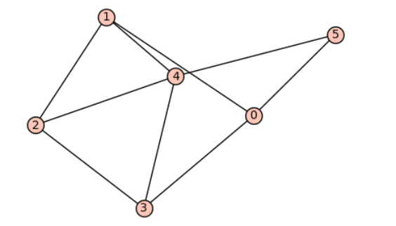
Now, let us execute the code to view the output. As before, we use the online tool called CoCalc to do so. Log on to the CoCalc platform, type the code in the window, and save it as ‘graph3.sagews’. Then, press the Run button to execute the code. Figure 1 shows the graph called Graph_3 generated by the above code on execution. It can be seen that Graph_3 is isomorphic to Graph_1 constructed in the previous article. Two graphs are called isomorphic if they are ‘somewhat’ equal. Please refer to the second article in this series for a more detailed explanation of isomorphic graphs.
Now, we construct a graph (which we will call Graph_4) using an incidence matrix with SageMath. The SageMath code, saved as ‘graph4.sagews’, is provided below (line numbers have been included for clarity in the explanation).
1.	from sage.graphs.graph import Graph
2.	inc_matrix = [
	    [1, 1, 1, 0, 0, 0],
	    [1, 0, 0, 1, 0, 0],
	    [0, 1, 0, 1, 1, 0],
	    [0, 0, 1, 0, 0, 1],
	    [0, 0, 0, 0, 1, 1]
	]
3.	G = Graph( )
4.	num_vertices = len(inc_matrix)
5.	num_edges = len(inc_matrix[0])
6.	for i in range(num_vertices):
7.	    G.add_vertex(i)
8.	for j in range(num_edges):
9.	    edge=[ ]
10. 	    for i in range(num_vertices):
11.               if inc_matrix[i][j] == 1:
12.                   edge=edge+[i]
13.               G.add_edge(edge[0],edge[1])
14.	G.show( )
Now, let us go through the code for better understanding. As before, Line 1 imports the Graph class from the sage.graphs.graph module. Line 2 stores the incidence matrix of the graph into the variable inc_matrix. Line 3 creates an instance of the Graph class, initialising an empty graph to the variable G. Line 4 calculates the number of vertices in the graph by finding the length of the incidence matrix, which is the number of rows. Line 5 calculates the number of edges in the graph by finding the length of the first row of the incidence matrix, which is the number of columns. The for loop in Line 6 iterates over the vertices of the graph. For each vertex index i, Line 7 adds a vertex to the graph. The for loop in Line 8 iterates over the edges of the graph. Line 9 initialises an empty list named edge to store the vertices incident to the current edge. The nested for loop in Line 10 iterates over the vertices of the graph again. The condition in Line 11 checks if vertex i is incident to edge j by examining the corresponding entry in the incidence matrix. If vertex i is incident to edge j, its index is added to the list named edge in Line 12. After identifying the two vertices incident to edge j, Line 13 adds an edge between them to the graph. Finally, Line 14 displays the constructed graph.
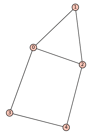
Now, let us execute the code to view the output. Use CoCalc to run the program named ‘graph4.sagews’. Figure 2 shows the graph called Graph_4 generated by the above code on execution. It can be seen that Graph_4 is isomorphic to Graph_2 constructed in the second article in the series.
Now that we are familiar with creating graphs using different methods that suit our needs, let us discuss some methods provided by SageMath to elicit more information from the graphs we have constructed. I will also introduce some graph theoretic terminology as and when required. In order to enhance clarity, I have occasionally opted for simplicity over strict mathematical rigour. As a result, some of the definitions provided may not adhere strictly to textbook standards. However, they should still offer you a good grasp of the concepts we are covering.
There are hundreds of methods offered by SageMath just for processing graphs alone, and we will be discussing a few so that you have an idea about how to use them. First, let us discuss the all_paths( ) method, which will list all the available paths between a pair of vertices. Formally, a path in a graph is a sequence of vertices where each vertex is connected to the next vertex by an edge. Add the following line of code, which will list all the paths from vertex 3 to vertex 4, at the end of the program called ‘graph4.sagews’.
print(G.all_paths(3, 4))
Execute the program again, and it will print the following output below the image of the graph.
[[3, 0, 1, 2, 4], [3, 0, 2, 4], [3, 4]]
Though there is an edge between vertices 3 and 4 (a path of length 1), you can also reach 4 from 3 by going through vertices 0, 1, and 2 (a path of length 4), and by going through vertices 0 and 2 (a path of length 3). Hence, the output shows all three distinct paths from 3 to 4. Please find paths between other pairs of vertices as well to gain a better understanding of the situation.
Before we proceed further, let us try to understand what a cycle in a graph is. This is a path that starts and ends at the same vertex, and it doesn’t visit any vertex more than once, except for the starting and ending vertex, which are the same. I use the symbol em dash (—) to denote an edge between a pair of vertices, say 0 and 2, as follows: 0—2. If you observe Graph_2 shown in Figure 2, 0—2—1—0 is a cycle of length 3, also known as a triangle in graph theory. Notice that 2—1—0—2 and 1—0—2—1 are also the same as the cycle 0—2—1—0. Another cycle in Graph_4 is 3—0—2—4—3, which is a cycle of length 4. Surprisingly, there exists a cycle of length 5 also in Graph_4. That cycle is 3—0—1—2—4—3. The edge 0—2 is called a chord of this cycle. A cycle without a chord in the original graph is called an induced cycle. Now, add the following lines of code at the end of the program called ‘graph4.sagews’.
G.longest_cycle(induced=true)
G.longest_cycle(induced=false)
The above two lines of code print the number of vertices in the largest induced cycle and the largest cycle in the graph Graph_4. Upon execution, the following output is printed on the screen.
longest induced cycle: Graph on 4 vertices
longest cycle: Graph on 5 vertices
From the output, we can see that the longest induced cycle in Graph_4 contains 4 vertices, and thus the cycle is of length 4. The induced cycle of length 4 in Graph_4 is 0—2—4—3—0. Additionally, from the output, we can see that the longest cycle in Graph_4 contains 5 vertices, and thus the cycle is of length 5. The induced cycle of length 5 in Graph_4 is 0—3—4—2—1—0.
Now, let us try to elicit more useful information from graphs. First, let us try to understand what a Eulerian cycle is, which is named after the great Swiss mathematician Leonhard Euler. A Eulerian cycle is a cycle in which every edge is visited exactly once. What is the point of finding a Eulerian cycle in a graph? Well, let us assume the graph in consideration represents the road map of a city. If you are tasked with inspecting the quality of all the roads in the city, how will you proceed? Will you travel randomly, or will you have some strategy? Ideally, you would start from your office and inspect all the roads exactly once by travelling through them and coming back to your office at the end. This sort of cycle in a graph is called a Eulerian cycle. Of course, such a route may not be available in the graph (in this case, through the roads of the city). However, SageMath offers a method called eulerian_circuit( ), which will return a list of edges forming a Eulerian cycle if one exists. If no Eulerian cycle is found, the method returns False. Keep in mind that cycles are often called circuits in graph theory. Now, add the following line of code at the end of the program called ‘graph4.sagews’.
G.eulerian_circuit(labels=False)
Since there are no labels on the edges of Graph_4, the argument labels is set to False. Upon execution, the output shown on the screen is False. Therefore, there is no Eulerian cycle in this graph. Hence, while inspecting the roads, you will have to travel through at least one road twice. Now, let us check whether Graph_3 has a Eulerian cycle or not. Upon execution of the modified version of the program ‘graph3.sagews’, we can see that even Graph_3 does not contain a Eulerian cycle. Let us modify the program so that a new graph with a Eulerian cycle is created, thus allowing us to observe the output. Modify Line 2 of ‘graph3.sagews’ so that the adjacency matrix shown below is used to obtain a new program called ‘graph5.sagews’.
adj_matrix = [
    [0, 1, 0, 0, 0, 0, 0, 1],
    [1, 0, 1, 1, 0, 0, 0, 1],
    [0, 1, 0, 1, 0, 0, 0, 0],
    [0, 1, 1, 0, 1, 1, 0, 0],
    [0, 0, 0, 1, 0, 1, 0, 0],
    [0, 0, 0, 1, 1, 0, 1, 1],
    [0, 0, 0, 0, 0, 1, 0, 1],
    [1, 1, 0, 0, 0, 1, 1, 0]
]
Upon execution of the program ‘graph5.sagews’ we obtain the graph called Graph_5, as shown in Figure 3.
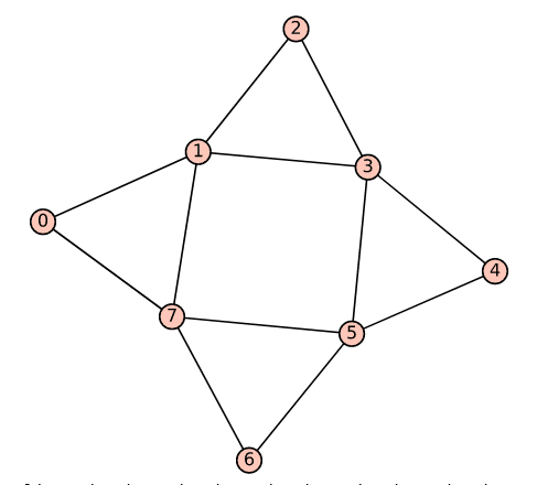
As I have already mentioned, Graph_5 contains a Eulerian cycle. Let us modify the program ‘graph5.sagews’ to check for a Eulerian cycle. Upon execution of the modified version of the program ‘graph5.sagews’, we get the following output displayed on the screen.
[(0, 7), (7, 6), (6, 5), (5, 4), (4, 3), (3, 5), (5, 7), (7, 1), (1, 3), (3, 2), (2, 1), (1, 0)]
It can be seen that the cycle 0—7—6—5—4—3—5—7—1—3—2—1—0 visits all the 12 edges in Graph_5 exactly once. Thus, it is a Eulerian cycle.
Now, let us discuss Hamiltonian cycles (named after the Irish mathematician William Rowan Hamilton) in a graph. This is a cycle in a graph where every vertex is visited exactly once. Under what circumstances does a Hamiltonian cycle come in handy in a real-life situation? Let us again consider the roads in a city. Assume this time you are tasked with inspecting the traffic lights at every junction in a city. Unlike the last time, you don’t have to visit every road in the city. Here, a Hamiltonian cycle becomes very useful. Ideally, you would only visit each junction in the city (each vertex in the graph) exactly once. Again, there is no guarantee that such a route exists. There are graphs where you need to visit certain vertices more than once. Let us first check Graph_5 for a Hamiltonian cycle. Add the following line of code at the end of the program called ‘graph5.sagews’.
G.hamiltonian_cycle(algorithm=’backtrack’)
The above line of code checks whether Graph_5 has a Hamiltonian cycle or not. The method returns True if there exists a Hamiltonian cycle in Graph_5 along with the actual Hamiltonian cycle vertices as a list, using a backtracking algorithm. It returns False if there exists no Hamiltonian cycle along with a list showing where the algorithm failed (in the sense that it recognised there exists no Hamiltonian cycle). Upon execution of the modified version of the program ‘graph5.sagews’, we get the following output displayed on the screen.
TSP from : Graph on 8 vertices
(True, [4, 5, 6, 7, 0, 1, 2, 3])
It can be observed that the cycle 4—5—6—7—0—1—2—3—4 is a Hamiltonian cycle. Now, let us check whether Graph_3 has a Hamiltonian cycle or not. Upon execution of the modified version of the program ‘graph3.sagews’, we get the following output displayed on the screen.
TSP from : Graph on 6 vertices
(True, [5, 4, 1, 2, 3, 0])
It’s clear that the cycle 5—4—1—2—3—0—5 is a Hamiltonian cycle. Recall that Graph_3 does not have a Eulerian cycle. Modify the program ‘graph4.sagews’ accordingly and verify that Graph_4, which does not have a Eulerian cycle, also has a Hamiltonian cycle. Thus, even if a graph does not have a Eulerian cycle, it still can contain a Hamiltonian cycle.
Now, we need to answer another question: If a graph has a Eulerian cycle, does it always have a Hamiltonian cycle? Let us modify Line 2 of the program ‘graph3.sagews’ so that the adjacency matrix shown below is used to obtain a new program called ‘graph6.sagews’.
adj_matrix = [
[0, 1, 1, 0, 0],
[1, 0, 1, 1, 1],
[1, 1, 0, 0, 0],
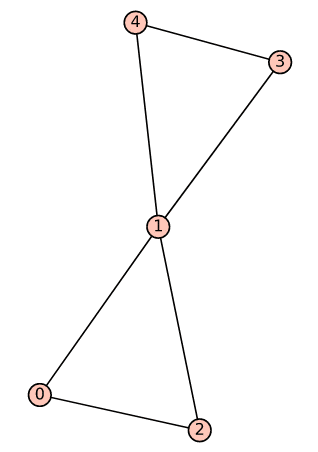
Upon execution of this program, we obtain the graph called Graph_6, as shown in Figure 4.
Now, add the following line of code at the end of the program called ‘graph6.sagews’ to check whether Graph_6 has a Eulerian cycle and a Hamiltonian cycle.
G.eulerian_circuit(labels=False)
G.hamiltonian_cycle(algorithm=’backtrack’)
Upon execution of the modified version of the program ‘graph6.sagews’, the following output is displayed on the screen.
[(0, 2), (2, 1), (1, 4), (4, 3), (3,1), (1, 0)]
(False, [0, 2, 1, 4, 3])
The cycle 0—2—1—4—3—1—0 visits every edge of Graph_6 exactly once and hence is a Eulerian cycle. Further, it has no Hamiltonian cycle. Thus, a graph not containing a Hamiltonian cycle can have a Eulerian cycle. As a further note, the problems of finding a Eulerian cycle and a Hamiltonian cycle form a very interesting class of problems in computer science. At a casual glance, the two problems look very similar; however, that is not the case. Finding a Eulerian cycle is a problem that belongs to a group of problems in class P, all of which have computationally feasible solutions. Finding a Hamiltonian cycle is a problem that belongs to a group of problems in class NP-complete, and so far, none of these have computationally feasible solutions. Whether problems in class NP-complete have computationally feasible solutions is one single greatest open problem (one of the seven Millennium Prize Problems selected by the Clay Mathematics Institute) in computer science. Any person who solves this problem will receive a Turing Award, Abel Prize, Fields Medal (if the person is under the age of 40), along with US$ 1 million from the Clay Mathematics Institute, and many more accolades.
So far, we have only generated undirected simple graphs (having at most one edge between a pair of vertices). Let us again consider the case of roads in a city. Suppose there are two parallel roads connecting two places in a city. How do we represent them in a graph? Here, multigraphs come to our help. A multigraph can have loops (edges starting and ending at the same vertex) and parallel edges (more than one edge between a pair of vertices). The program ‘mgraph7.sagews’ shown below generates a multigraph called Mgraph_7 (line numbers have been included for clarity in the explanation).
1. MG = Graph(multiedges=True, loops=True)
2. MG.add_vertices([1, 2, 3, 4])
3. for i in [1, 2]:
4. MG.add_edge(1, 2)
5. MG.add_edge(2, 3)
6. MG.add_edge(3, 4)
7. MG.add_edge(4, 1)
8. MG.add_edge(i, i)
9. MG.add_edge(i+2, i+2)
10. MG.show( )
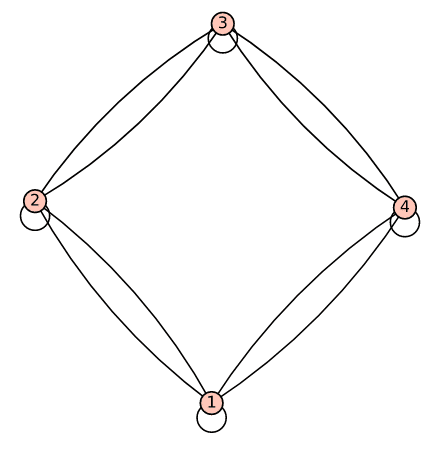
Now, let us go through the code for better understanding. Line 1 creates a new graph object called MG with the Graph( ) constructor. The argument multiedges is set to True, indicating that the graph can have multiple edges between the same pair of vertices. The argument loop is also set to True, indicating that the graph can have loops. Line 2 adds vertices labelled 1, 2, 3, and 4 to the graph. Line 3 starts a for loop that iterates over the values 1 and 2. Lines 4 to 7 add edges between vertices 1 and 2, 2 and 3, 3 and 4, and 4 and 1. Since the for loop iterates twice, two parallel edges are created between these pairs of vertices. Lines 8 and 9 create loop edges. On the first iteration of the for loop, loop edges are added to vertices 1 and 3. On the second iteration of the for loop, loop edges are added to vertices 2 and 4. Finally, Line 10 displays the graph. It will show all the edges, including loops and multiple edges, as configured in the graph creation step. Upon execution of the program ‘mgraph7.sagews’, we get the multigraph called Mgraph_7 shown in Figure 5.
Now, let us list all the loops in the multigraph Mgraph_7. To do that, add the following line of code at the end of the program called ‘mgraph7.sagews’.
MG.loops(labels=False)
Upon execution of the modified version of the program ‘mgraph7.sagews’, we get the following output. From the output, we can see that loops are created on vertices 1, 2, 3, and 4.
[(1, 1), (2, 2), (3, 3), (4, 4)]
Now, let us wrap up our discussion. In this third article in the series on SageMath, we explored various methods for creating undirected simple graphs. We also delved into techniques for extracting information from a graph when it represents a real-world problem in an abstract manner. Additionally, we examined the construction of multigraphs.
However, our exploration of graph theory in the context of SageMath is far from over. In the upcoming articles in this series, we will delve further into the topic of graphs. Why? Because graphs are an incredibly powerful data structure with applications in solving numerous real-world problems.


