

We explore the Java Vector API and its role in enabling data parallelism in Java applications by delving into its core concepts, including vectorization, Vector API components, and operations. The API’s ability to efficiently process data in parallel makes it ideal for tasks like scientific simulations, image processing, and machine learning.
Data parallelism is a critical technique for achieving high-performance computing in modern applications, especially those dealing with large data sets and computational workloads. The Java Vector API, introduced as part of Project Panama, represents a significant advancement in the Java ecosystem, providing developers with a powerful toolset to harness the full potential of data parallelism on multicore processors and vectorized hardware.
Java Vector API: What is it?
The Java Vector API aims to provide developers with a clear and concise way to express vector computations, which can be compiled at runtime by the just-in-time (JIT) compiler, into optimal vector instructions on supported CPU architectures. It enables programmers to write code in Java that can express complex data parallel algorithms and help achieve performance superiority to equivalent scalar or sequential computations.
These APIs were introduced in JDK 16 and are currently in the eighth phase of incubation in the recently introduced Java 23. They should soon move out of the incubation phase and into a preview state in an upcoming Java version.
Auto vectorization
The JIT-compiler tries to optimise the compilation of the byte code with loop optimisations, inlining and emit vectorized SIMD instructions supported by the underlying platform. This technique is called auto vectorization by the JIT compiler in Java.
Auto vectorization is attempted for the cases where the compiler can find opportunities for optimisations. Usually, these are simple blocks/snippets in the code which the compiler can easily recognise for optimisation based on JIT compiler profiling at various stages of dynamic compilation.
Some would argue that we do not need Java Vector API when we already have ‘auto vectorization’ from the JIT compiler. Sure, we do, but it is not always guaranteed and is based on dynamic profiling of byte code by JIT. These APIs can be utilised to exploit the inherent platform potential while processing huge data sets in OLAP/Big Data applications. These APIs are most efficient especially for data parallel algorithms, and guarantee the execution in vectorized hardware supported by the underlying platform.
Intrinsics in the C++ world
In the C++ world, intrinsics are used for parallelism. These are a set of functions or instructions that allow developers to incorporate processor-specific instructions directly into their code. They can be used in C++ to force vectorization when auto vectorization is insufficient, but are platform-specific, so the same code may not be compatible with other platforms.
The Java Vector API offers a distinct advantage over this approach. It eliminates the need for such forced interventions by doing the heavy lifting itself, ensuring that your code is efficiently vectorized and uses platform-specific vector instructions in a more powerful way at runtime during its JIT compilation. Java’s portability, ‘write once and run anywhere’, is greatly complemented by the Vector API, as it adapts to different hardware architectures due to JIT compilation at runtime, while maintaining efficient vectorized operation.
Where does Java Vector API fit in?
Instruction-level and bit-level parallelism are inherent to the hardware. Their efficiency depends on factors like the sophistication of the branch prediction algorithm and the design of the pipelining process in CPU microarchitecture. These hardware-specific features vary from one platform to another and are not typically accessible through open APIs for developers.
Data and task parallelism are accessible within the programming language, and developers can use specific APIs to leverage these forms of parallelism. Task parallelism can be achieved in Java using the concurrency and multi-threading APIs in the java.util.concurrent package of Java.
Application-level performance in multi-core systems can be optimised through data parallelism using the single instruction, multiple data or SIMD approach. There are platform-specific instructions called SIMD instructions that can enable data parallelism. As these are different for different hardware, they become tedious to keep track of. Java Vector API sweeps in and acts like a diplomat between the underlying platform-specific code and the high-level Java code, which is easy to understand and implement, keeping Java’s portability philosophy of ‘write once and run anywhere’ intact.
| Back to the basics |
|
What is parallelism? Parallelism simply means performing tasks simultaneously. Parallel computing uses multiple processing elements, wherein each processing element executes a part of the complex large problem simultaneously. The aim of parallel computing is to achieve faster computational performance with efficient utilisation of available resources like CPUs or GPUs (muti-processors/multi cores), memory (registers/cache/RAM), etc. It can be done at different levels which brings us to its types: data parallelism, task parallelism, bit-level, instruction level, and hybrid parallelism. 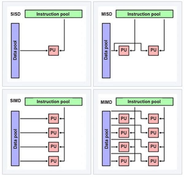 Data parallelism involves processing large data sets by applying the same function across subsets. It involves synchronous processing where performance scales with the amount of data processed — more data means better performance. This approach is very apt in scenarios where the data under processing is homogenous and data dependency between the operations is not involved with previous operations. It’s mostly used in media data like audio/video processing, machine learning and distributed databases. Task parallelism breaks down large tasks into smaller, parallel-executable subtasks. In contrast with data parallelism, task parallelism is characterised by asynchronous processing, which necessitates managing concurrency (for interdependent data). For instance, multi-threading is an important form of parallelism, wherein programs are divided into threads (small tasks) that share single or multiple cores and other resources like caches and buffers. Bit-level parallelism refers to the evolution of processor word length. Historically, processor support has progressed from 8-bit to 16-bit, to 32-bit, and now to 64-bit processors. Bit-level parallelism is the capability to process a larger word length in a single instruction or cycle. The more support there is at the bit level, the fewer instructions are required to process data. Bit-level parallelism is commonly used in digital signal processing, cryptography, and arithmetic calculations. Instruction-level parallelism allows for the execution of multiple instructions simultaneously. For any instruction to run, it typically goes through fetch, decode, and execute steps. Using pipelining techniques, these steps can be parallelised, enabling simultaneous processing of instructions. There are sophisticated branch prediction techniques that enable the pre-fetching of the next instruction well ahead of its execution to improve instruction processing. Hybrid parallelism is a blend of all these elements. Based on specific needs, one can combine data parallelism and task parallelism with instruction-level parallelism. The end user’s experience can be optimised integrating the strengths of each type of parallelism. Flynn’s taxonomy Based on how instructions and data are used in parallel, Flynn’s taxonomy categorises computer architectures into four primary types: SISD, MISD, SIMD, and MIMD. This framework illustrates how different architectures approach parallel processing. SISD (single instruction, single data stream) involves applying a single instruction to a single data stream to produce one result. It’s good for primitive uniprocessors, which execute instructions sequentially. MISD (multiple instruction, single data stream) involves executing multiple instructions on a single data set. Its practical applications are very limited. MISD can be used in contexts like evaluating fault tolerance, where multiple instructions are executed on the same data to verify the correctness of the results. SIMD (single instruction, multiple data) involves a single operation being performed on multiple sets of data, known as data parallelism. Here the instruction is broadcast to all processing units, and each unit independently performs the same operation on different pieces of data simultaneously. All modern processors and GPUs have support for this kind of processing using vector instructions extensions. SIMD processors are often referred to as vector processors. MIMD (multiple instruction, multiple data) involves applying multiple instruction operations to multiple data points within a data set. Supported by many of the latest processors, this approach leverages computer hardware to use multiple instructions on a larger data set. |
Data vectorization using SIMD
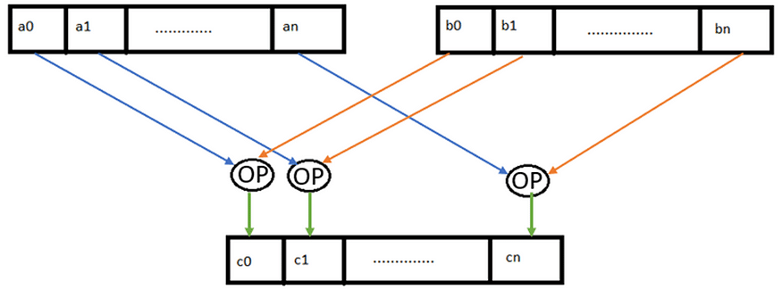
SIMD is a computing method using which a single operation, such as an arithmetic operation or a complex operation like fused multiply-add (FMA), is applied across two vectors (sets of data points and not single data points). SIMD instructions of the underlying platform are used to achieve data parallelism. Here the vector registers, supported by the underlying platform, are utilised to realise data parallelism.
In a sequential or scalar approach, each data element is processed one at a time. While, in a single instruction cycle, SIMD can execute operations on multiple data elements simultaneously, improving efficiency and reducing costs.
An important aspect of SIMD is data independency — one iteration should not affect the outcome of another and the data being operated on should be homogenous in nature.
Components of Java Vector API code
Java Vector API provides platform-agnostic ways for Java developers to write data parallel algorithms without necessarily knowing the specifics of that hardware. It is the JIT compiler’s responsibility to then translate the high-level Java Vector API code into appropriate SIMD instructions to leverage the hardware capabilities at runtime. The constructs in Java Vector APIs that developers can use to write data parallel algorithms are discussed below.
- Vector shape
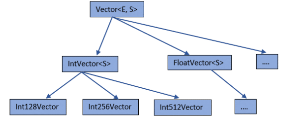
Vector shape refers to the bit width a specific platform can support. Each platform has its limitations regarding how many bits it can handle in a single vector operation, based on its support of vector registers. This bit width of the vector registers determines the amount of data that can be processed in parallel in a single vector instruction. For example, a platform supporting a 512-bit width register can handle more data elements processing simultaneously compared to a platform with a lower bit width support. The API to get the underlying platform’s default shape supported is VectorShape.preferredShape(). It can be either 64, 128, 256 or 512-bit width based on the underlying platform. - Vector species
Vector species is a combination of a data type (like int, float, etc) and the vector shape (bit width). Each element within a vector is referred to as a ‘lane’. So, the number of lanes that can be accommodated in a vector is determined by the vector species.
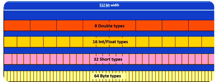
For example, the Float Vector of Species ‘VectorSpecies<Float> SPECIES_512’ can fit 16 floats (16 lanes of float type; 512-bit width/32-bit float size = 16 floats). Figure 4 shows the number of lanes supported for a platform, which support a 512-bit wide vector register for each data type.
For every data type we can get the preferred vector supported by the platform using the ‘SPECIES_PREFERRED’ defined in the respective data type vector. For example, for float type we can get the float species preferred by the platform using the following:
VectorSpecies<Float> preferredSpecies = FloatVector.SPECIES_PREFERRED;
Let us now understand how to write simple vector code by taking an example provided in the JEP proposal of Vector API.
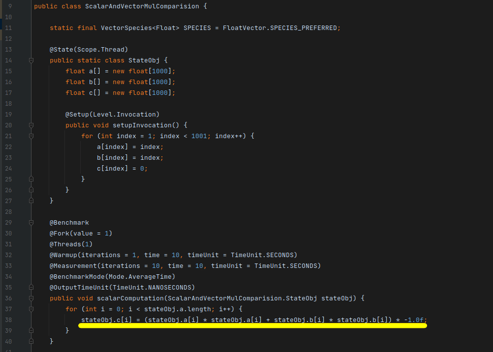
Consider two float arrays and an operation involving the addition of the squares of two numbers, followed by their negation. In Figure 5, a basic scalar operation — a non-vectorised, sequential code has been implemented (simply ((a2 + b2 ) * (-1)) ).
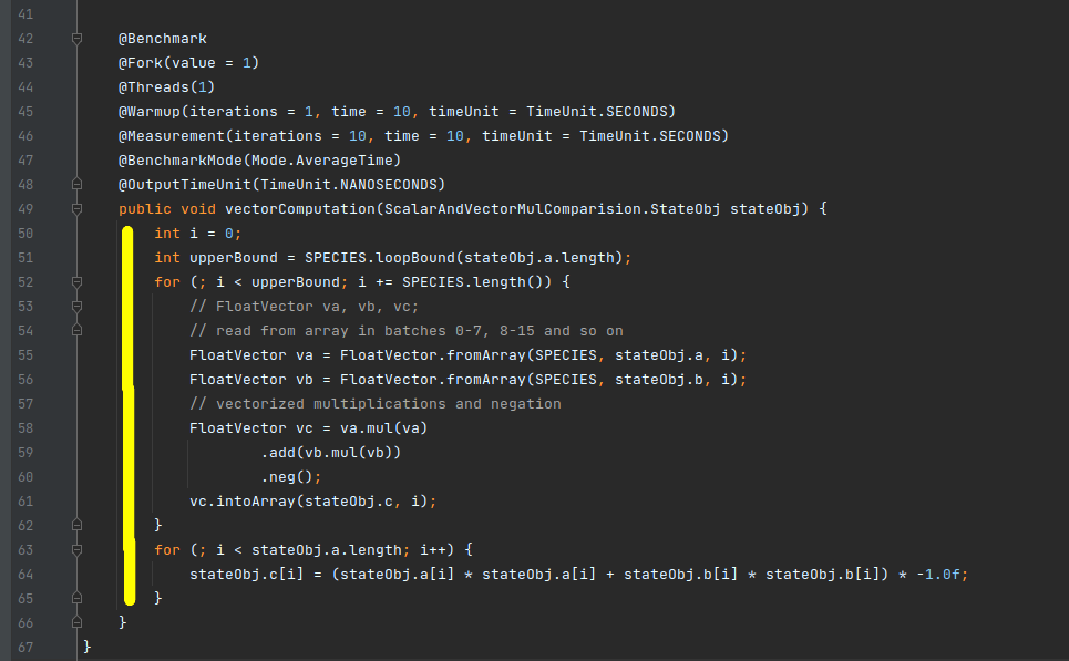
In Figure 6, the vector code has been implemented. The vector species provides an API called ‘loopBound’, which returns the maximum iterations that can be performed in a vectorized manner for the total provided iterations. Considering that FloatVector.Species_512 can support sixteen floats at a time, for 10000 iterations the loopBound API for FloatVector.Species_512 returns 625 (10000/16). Here, we can fit all the data in vectorized processing for 10000 float elements into 625 vectorized iterations (line number 52 to 61).
Let’s take another example where we must process only 36 float values instead of 10000. The loopBound API will return 2 (36/16 = 2.xx), meaning 2 iterations can be performed in a vectorized manner handling 16 floats at a time, in a total of 32 floats. The remaining 4 floats, which do not fit into the vectorized flow, should be handled in a scalar or sequential manner as seen from line number 63. This section of the code, which handles the remaining data elements that don’t qualify for vectorized computation, is called the ‘tail part’.
The process involves reading from the array into vectors one at a time — from indices 0 to 15, then 16 to 31, and so on. The calculations, including multiplications and negation, are then performed in a vectorized, data-parallel manner, which is more efficient than executing them sequentially. The results are stored back into the resultant array or vector, denoted as ‘vc’.
| Optimisations using Java Vector API |
|
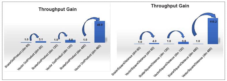
Speeding up Lucene vector similarity through the Java Vector API In Figure 8, ‘dim’ is the dimension/length of the float[] arrays in test and ‘score’ is the number of dot product/Euclidean distance operations done per second. ‘Gain’ is the increase in speed of the vectorized implementation against the corresponding default implementation. Lucene is a search engine library used in applications like Elasticsearch, OpenSearch, and Solr. Approximate nearest neighbour (ANN) search was introduced in Lucene 9. Calculating distances (dot-product, Euclidean distance, and cosine) between two vectors in vector space is a compute-intensive task. Lucene’s implementation of ANN relies on a scalar implementation of the vector similarity functions ‘dot-product’, ‘Euclidean distance’, and ‘cosine’. Distance calculation can be increased multi-fold by vectorizing the scalar implementation. As the dimensions increase, the performance gains from vectorization increase, improving by ~50 times and ~115 times for dot product and square distance computations, respectively. With vector dimensions of 300 or higher, the efficiency gains are even more significant (do refer to Lucene JIRA #12091). JavaFastPFOR optimisation JavaFastPFOR is a library designed for the efficient compression and decompression of integers. This library is well-regarded and used within Apache Pinot, a real-time distributed OLAP datastore, and is already incorporated into the file format, Parquet. The VectorJavaFastPFOR (re-written with Java Vector API) algorithm compresses integers in blocks of 256 integers and provides a promising performance benefit ranging from around 4x to 10x improvements for vectorized implementations. There is also a proposal (Lucene JIRA #12090) for integration of this library within Lucene’s posting file format. |
Vector operations: Lane-wise vs cross-lane
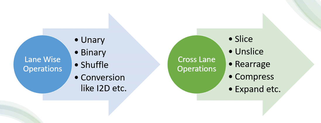
The Java Vector API supports multiple operations and functions, with the concept of a ‘lane’. These operations can be categorised based on the resultant lane length as lane-wise and cross-lane operations.
When an operation produces a result with the same length as the input vectors, it is referred to as a lane-wise operation. It yields results with the same lane count as the source vectors. Lane-wise operations include unary, binary, shuffle, and conversions like I2D, etc.
In addition to lane-wise operations, there are also cross-lane operations. These may result in vectors with a lesser lane count than the source vectors, depending on how the operation consolidates or processes the data across lanes. Slice, unslice, rearrange, compress, and expand, etc, are cross-lane operations.
Graceful degradation
Taking into consideration that everything has its limitations, the Java Vector API aims to degrade gracefully. What does this mean?
Although the aim is to make vector calculation platform-independent, sometimes, the high-level language vector instructions may not be compiled by the JIT compiler to optimise vector instructions they are supposed to. This could be because they are not supported on that hardware, or because of some limitation of the JIT compiler to emit vectorized instructions in certain specific cases. In such cases the Vector API implementation should degrade gracefully and still work. This means that the result produced should still be the same as in the case of non-vector scalar implementation (like we do without vectors using, say, the ‘for’ loop). This is termed graceful degradation in Java Vector API.
This article is based on a joint speaking session by Sourav Kumar Paul, engineering manager at Intel, and Abhijit Kulkarni, senior software engineer, Intel, at Open Source India 2023.
Compiled by Shivangi Kharoo, tech journalist.


