Using R to Analyse an IoT Connected Health Monitoring System

We delve into the deployment of IoT for health monitoring using the statistical programming language R. The primary aim of the system developed here is to harness R’s analytical prowess to process and analyse real-time health data acquired from diverse IoT devices.

The health monitoring system proposed here incorporates wearable sensors, mobile applications, and cloud-based infrastructure to establish a seamless connection between individuals and healthcare providers. Wearable devices, equipped with sensors, continuously capture vital health metrics such as heart rate, blood pressure, temperature, and activity levels. These metrics are transmitted to a central server via the internet, where R-based algorithms are utilised for real-time analysis.

R plays a pivotal role in the processing of raw health data, execution of statistical analyses, and generation of meaningful insights. Leveraging the language’s extensive library of statistical functions, visualisation tools, and machine learning capabilities facilitates the development of predictive models aimed at identifying potential health issues. Additionally, R enables the creation of personalised health profiles and trend analyses for individuals, fostering proactive healthcare management. The architecture also encompasses a user-friendly mobile application, providing individuals with real-time access to their health information.

The application described here delivers personalised feedback, health recommendations, and alerts based on the analyses performed by R. Moreover, healthcare providers can remotely monitor patients’ health status and intervene promptly if anomalies are detected.

To ensure the security and privacy of health data, the system incorporates robust encryption and authentication mechanisms. The cloud-based infrastructure, leveraging R, ensures secure data storage and compliance with healthcare data protection regulations.

This proposed IoT connected health monitoring system exemplifies the substantial contribution R can make to the evolving field of digital healthcare. The objective of this system is to formulate an IoT based healthcare application that can predict the possibility of a heart attack through smart wearables, using generalised linear models (GLMs), random forests and decision trees in R.

The problem statement

The diagnosis of heart disease is a difficult task, but automation leads to better predictions about a patient’s heart condition. Data relating to resting blood pressure, cholesterol, age, sex, type of chest pain, fasting blood sugar, ST depression, and exercise-induced angina can all help to predict the likelihood of having a heart attack. Decision trees, random forests and GLMs can be trained on the given dataset and be used to view the predicted classes, where 0 equals less chances and 1 equals more chances of a heart attack.

Setting up the health monitoring system

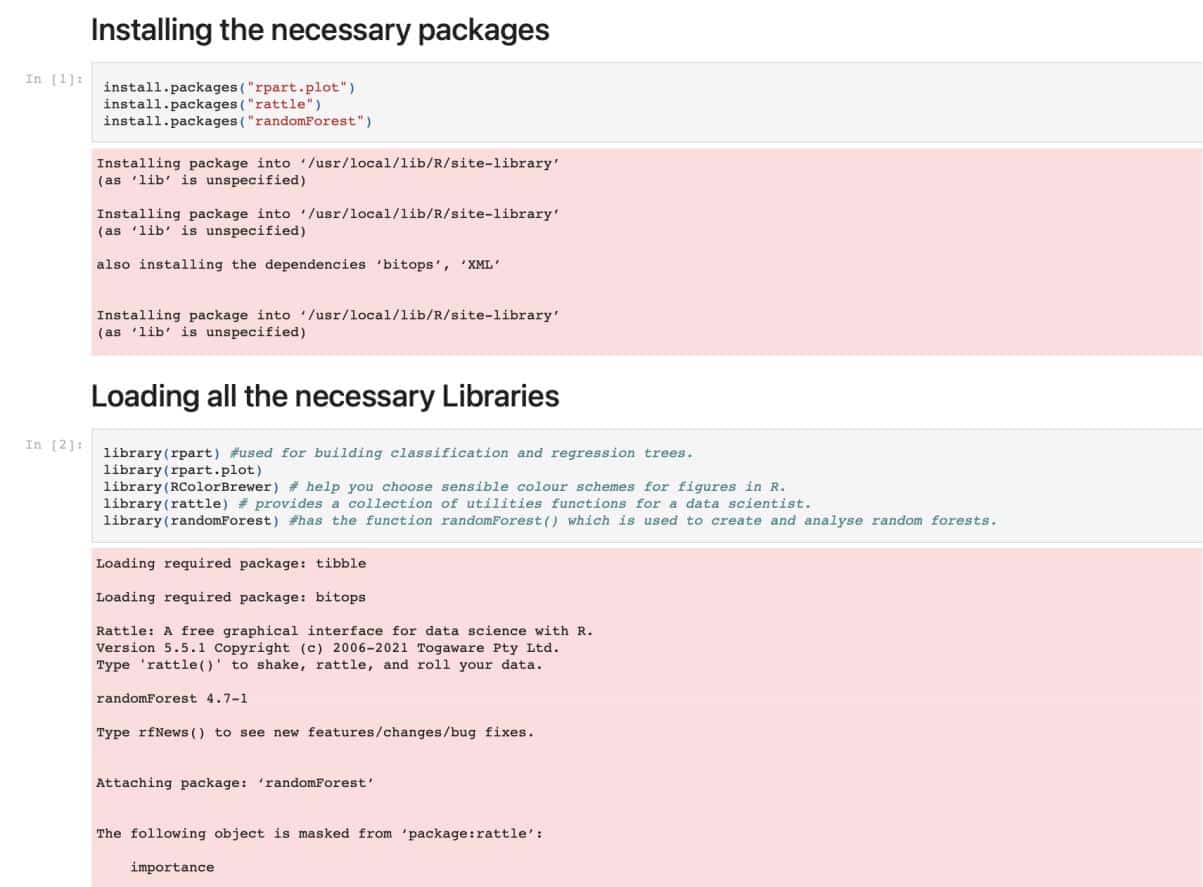
• Import the packages Rplot, RColorBrewer, Rattle and randomForest.
• Download and read the dataset from Kaggle at https://www.kaggle.com/ datasets/nareshbhat/health-care-data-set-on-heart-attack-possibility.
• View the statistics of the variables in the dataset using the function ‘summary’.
• Analyse the data, specific to resting blood pressure.
• Using the ‘cor’ function, find the correlation between resting blood pressure and age.
• Construct a logistic regression model using a GLM and view the output plots.
• Encode the target values into categorical values.
• Split the dataset into training and testing data in the ratio 70:30.
• Construct a decision tree model.
• Target variable is categorised based on resting blood pressure, serum cholesterol and maximum heart rate achieved.
• Plot the decision tree and view the output.
• Devise a random forest model based on the relationship between resting blood pressure, old peak blood pressure and chest pain type.
• View the confusion matrix and importance of each predictor.

The required data is fetched from the patient through IoT based smart wearables and is processed using the R tool. We will be using R version 3.3.2 (2016-10-31) and RStudio version 1.2.1335 here.

Now, load all the necessary libraries:

library(rpart) #used for building classification and regression trees.
library(rpart.plot)
library(RColorBrewer) # help you choose sensible colour schemes for figures library(rattle) # provides a collection of utilities functions for a data scientist. library(randomForest) #Used to create and analyse random forests.

Figure 1 shows the installation and loading of all the necessary packages.

Next, load the dataset:

data = read.csv(“heart_health.csv”)

Make the dependent variable a factor (categorical):

data$target = as.factor(data$target)

Now split the dataset into ‘test’ and ‘train’:

print(“Train Test Split”) # 70/30 Split
dt = sort(sample(nrow(data), nrow(data)*.7)) train<-data[dt,]
val<-data[-dt,] nrow(train) nrow(val)

Figure 2 represents the partitioning, i.e., the splitting of the dataset into train set and test set in a 70 to 30 ratio, respectively.

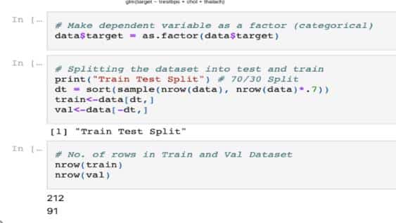
Figure 3 helps understand the dataset being considered for the health analysis case study.

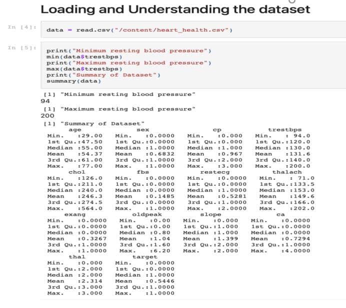
To analyse the data in the dataset, type:

print(“Minimum resting blood pressure”) min(data$trestbps)
print(“Maximum resting blood pressure”) max(data$trestbps)
print(“Summary of Dataset”) summary(data)

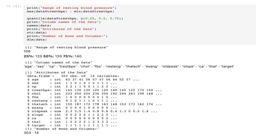
To arrive at the range of resting blood pressure, use the following code:

print(“Range of resting blood pressure”) max(data$trestbps) - min(data$trestbps) quantile(data$trestbps, c(0.25, 0.5, 0.75)) print(“Column name of the Data”) names(data)
print(“Attributes of the Data”) str(data)
print(“Number of Rows and Columns:”) dim(data)

Figure 4 captures the range of resting blood pressure for the health analysis case study.

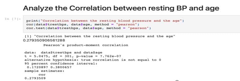
To analyse the correlation between resting BP and age, use this code snippet:

print(“Correlation between the resting blood pressure and the age”)
cor(data$trestbps, data$age, method = “pearson”)
cor.test(data$trestbps, data$age, method = “pearson”)

Figure 5 gives the correlation between resting BP and age.

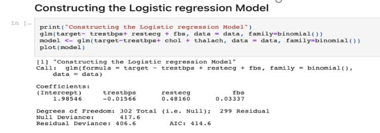
To construct the GLM, type:

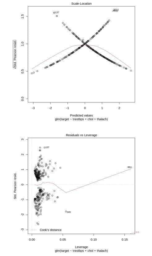
print(“Constructing the Logistic regression Model”)
glm(target~ trestbps+ restecg + fbs, data = data, family=binomial())
model <- glm(target~trestbps+ chol + thalach, data = data, family=binomial())
plot(model)

The outcomes of the construction of the logistic regression model are illustrated in Figure 6.

Use the following code to construct the decision tree model:

print(“Construction of the Decision Tree Model”) mtree <- rpart(target ~ trestbps + chol + thalach, data = train, method=”class”, control = rpart.control(minsplit = 20, minbucket = 7, maxdepth = 10, usesurrogate = 2, xval =10))

Now plot the decision tree for the dataset, using ‘mtree’:

print(“Plotting the Decision Tree”)

plot(mtree)

text(mtree)

par(xpd = NA, mar = rep(0.7, 4)) plot(mtree, compress = TRUE)

text(mtree, cex = 0.7, use.n = TRUE, fancy = FALSE, all = TRUE) prp(mtree, faclen = 0,box.palette = “Reds”, cex = 0.8, extra = 1)

Next, construct the random forest model:

rf <- randomForest(target ~ trestbps + oldpeak + cp, data = data)

View the forest results:

print(“Random Forest Results:”)
print(rf)

The importance of each predictor can be gauged by:

print(“Importance of each predictor:”) 
print(importance(rf,type = 2))

To plot the random forest, type:

plot(rf)

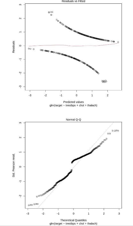
The graphical outcomes of the regression model are depicted in Figures 7 and 8.

This IoT-based healthcare application for predicting the possibility of a heart attack using GLMs, random forests, and decision trees in R holds significant promise for predictive healthcare analytics. The GLM, as implemented in R, offers a robust foundation for predicting heart attack probabilities based on a variety of input features. Its flexibility in handling different types of response variables and accommodating complex relationships between predictors enhances the accuracy of risk predictions.

The integration of random forest in the healthcare application further enhances this accuracy. Random forest leverages multiple decision trees, leading to a more robust and accurate prediction model. It can handle high-dimensional data and capture intricate patterns in the dataset.

Similarly, the inclusion of decision trees provides interpretable and actionable insights into the decision-making process. Decision trees, when used in conjunction with IoT data, allow for the identification of critical features influencing heart attack risks. The simplicity and transparency of decision trees facilitate the communication of results to both healthcare professionals and individuals.

In IoT-based healthcare, the collaborative use of GLMs, random forests, and decision trees in R synergises the strengths of these models to create a comprehensive predictive framework. The combination of these techniques not only enhances accuracy but also provides a holistic view of the potential risk factors associated with heart attacks.