Building Machine Learning Models with TensorFlow

This article offers an insight into machine learning models and how TensorFlow can be used to build them.

Machine learning is a young technology and is characterised by software that learns from past experiences to improve a system’s performance. It is the most efficient way to develop an algorithm that translates its input to the related output.

For example, consider a series of numbers denoting a gray scale image as an input. It is difficult to write an algorithm to label each and every object of an image. This is where machine learning is so useful. It provides a toolset to read and write software without describing every detail of the algorithm. If the developer leaves some ambivalent values, machine learning will automatically figure out the best output by itself.

These ambivalent values are also called parameters, and their description is referred to as a model. The user’s work is to write an algorithm that observes past examples to figure out how to tune parameters to achieve the model in an efficient way.

Learning and inference

Machine learning algorithms are examined in two ways: learning and inference. The prime aim of the learning step is to describe the data, which is called a feature vector, and aggregate it in a model. The learning algorithm selects a model and actively searches for this model’s parameters. This stage is more time consuming. The inference step moulds the model created in the learning step into an intelligent model.

Data representation, features and vector norms

The feature vector is a practical specification of data. To find out the accuracy of the real world data, the number of dimensions in the feature vector is included and the similarity is calculated by distance metrics (comparing similarity between the objects is an essential step in machine learning).

Let’s take two feature vectors a=(a1, a2,…..an) and b=(b1,b2,…..bn). The Euclidean distance || a-b || is calculated by:

The learning approach generally follows the structured models. Primarily, the data set needs to be transformed into a representation, which includes the everyday list of features and, finally, it can be used by the learning algorithm.

The inference process takes less time and can be faster when it works with real-time data. Once the process ends, the inference tests the model on new data.

Types of machine learning

There are three types of machine learning:

• Supervised learning
• Unsupervised learning
• Reinforcement learning

Supervised learning needs labelled data to implement a model. A model is just a function that labels data, including the past experiences. This is done with the help of past examples, which is denoted as a training data set.

The simple way to implement a model is through mathematical symbols. Let us consider ‘I’ to be an instance of data such as a feature vector. The related label associated with ‘I’ is ‘f(I)’. We can use the term ‘y=f(I)’ because it is easy to write. In context with any other example of classification, ‘I’ is a hundred-dimensional vector of different related vectors and ‘y’ is a pair of values that represent an outcome.

The model prediction of ‘I’ is denoted as ‘g(I)’. The model will have parameters that can be used and modelled either by humans or automatically. The parameter is represented by a vector ‘θ’. The combination of all these, ‘g(I|θ)’, represents a model.

Unsupervised learning models the data without labels or responses. Machine learning uses two powerful tools that learn from data alone — clustering and dimensionality reduction. Clustering is the process of collecting and dividing data into groups of similar items. Dimensionality reduction is used to manipulate data in order to view it in an easier way.
Reinforcement learning interacts with the environment to learn which pair or collection of action leads to an efficient outcome.

Machine learning uses powerful tools that are standardised, robust, and have high performance and scalability. This is where TensorFlow comes into the picture.

TensorFlow essentials

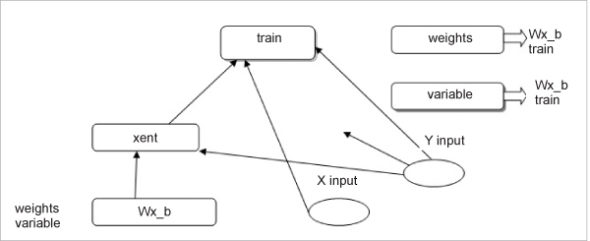
The machine learning framework created by Google is TensorFlow. This is used to “design, build and train machine learning models.” TensorFlow uses various libraries to do numerical computations, which are executed with a data flow graph. The graph contains nodes and edges, where nodes represent “mathematical operations and edges represent the data, which are generally multi-dimensional arrays or tensors, which are communicated between the edges.” TensorFlow enables developers to develop and deploy the models with ease and use them in machine learning. Automatic differentiation is one of the important properties of TensorFlow, since it makes it easier to implement the neural network concept of back-propagation.

Feature vectors are used predominantly in machine learning. A matrix represents a list of vectors, in which every bit of data contains a feature vector. Every column of a matrix represents a feature vector.

The syntax to represent a matrix is a vector of vectors in TensorFlow with the same length. The syntax for a tensor is nested vectors. The notion of scalar is rank 0 tensors, rank 1 tensors (i.e., vectors) and rank 2 tensors (i.e., matrices).

TensorFlow’s main data structure — tensors

Data management in TensorFlow is based on ‘tensors’. The fundamental concept of tensors “originates from the field of mathematics which is developed as a generalisation under the category of linear algebra in terms of vectors and matrices.” A tensor is described as a typed, multi-dimensional array with added operators modelled into the tensor object.

TensorFlow uses tensor data structure for representing all the data, since only the objects of the tensor type will be passed between the nodes in the computation graph.

Properties of tensors

Tensor rank: The dimensional aspect of a tensor is represented by tensor rank, which is different from a matrix rank. It represents the “quantity of dimensions” in which the tensors live. A rank 1 tensor is equivalent to a vector and comprises a matrix too. For a rank 2 tensor, any component can be approached with the syntax t[i, j]. For a rank 3 tensor, you will need to address a component with t[i, j, k], and so on.

Tensor shape: There is always a distinct connection between tensors and shapes. Rank 1, rank 2, rank 3 tensors have a shape of dimension 1, dimension 2 and dimension 3, respectively. An alternate way to represent a rank 3 tensor is a list that contains “matrices with the same shape.”

Tensor types: Tensors are of different types such as tf.float32, tf.float64, tf.int32, and tf.int64.

Handling the computation workflow

TensorFlow always behaves imperatively. It is recommended to install it under Anaconda Python.

Initialize interactive TensorFlow session
>>> import tensorflow as tf
>>> tf.Interactive Session()
<tensorflow.python.client.session. InteractiveSession>
Create a zeros tensor
>>> tf.zeros(2)
<tf. Tensor ‘zeros: 0’ shape=(2,) dtype=float32>
Evaluate the value of tensor
>>> a = tf.zeros(2)
>>> a.eval0
array([ 0., 0.], dtype=float32)
Creating constant tensors
>>> a = tf.constant(2)
>>> a.eval()
2
Creating identity matrix
>>> a= tf.eye(4)
>>> a.eval()
array([[ 1., 0., 0.. 0.],
[ 0.,1., 0., 0.],
[ 0.,0., 1., 0.],
[ 0.,0., 0., 1.]], dtype=float32)
Creating diagonal matrix
>>> r = tf.range(1, 5, 1)
>>> r.eval()
array([1, 2, 3, 4], dtype=int32)
>>> d = tf.diag(r)
>>> d.eval()
array([[1, 0, 0, 0],
[0, 2, 0, 0],
[0, 0, 3, 0],
[0, 0, 0, 4]], dtype=int32)

Visualising data using TensorBoard

TensorBoard is a software utility that accepts the graphical representation of the data flow graph. The interpretations of the results are handled by the dashboard.

To launch TensorBoard, type <url>:6006 into the Web browser. You can run it by using the command given below on a Windows computer:

<base> C:\Users\Administrator>tensorboard-logdir-summaries

TensorBoard 1.13.1 at http://SK-DK-24:6006 (Press CTRL+C to quit>

Let’s now attempt to build machine learning models with TensorFlow.

Linear and logistic regression with TensorFlow

Functions and differentiability are the basic concepts we need to know in order to understand machine learning. A function ‘f’ is a protocol that accepts an input to an output. A mathematical function is generally applied in basic physics and engineering. Differentiability is another type of control on functions. The fundamental advantage of the differentiable function is to use the slope of the function at a corresponding position to find out the places where the function is higher or lower than the present position. This helps to find out the minima of the function. For instance, if the function is at a higher level, the machine learning problems are solved by the loss function, where the minima of the function is encoded with real world problems to provide solutions.

A regression function generally uses L2 loss where the magnitude of a vector is measured.

Here, x is a vector of length N and L2 norm is generally defined as the distance between two vectors.

Let’s suppose that ‘a’ is a group of data, ‘b’ represents the corresponding labels, and ‘f’ is the differentiable function that encrypts the machine learning model. Since ‘f’ creates a prediction of ‘b’, then the L2 loss function will be determined as:

L(a,b) = || f(a)-b||2

Learning with TensorFlow

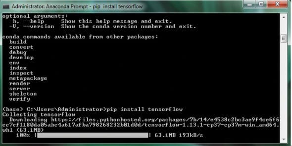
To install TensorFlow, use the command line:

C:\Users\Administrator\pip install tensorflow

Use the command given below to install Jupyter Notebook:

<base> C:\Users\Administrator\pip install jupyter

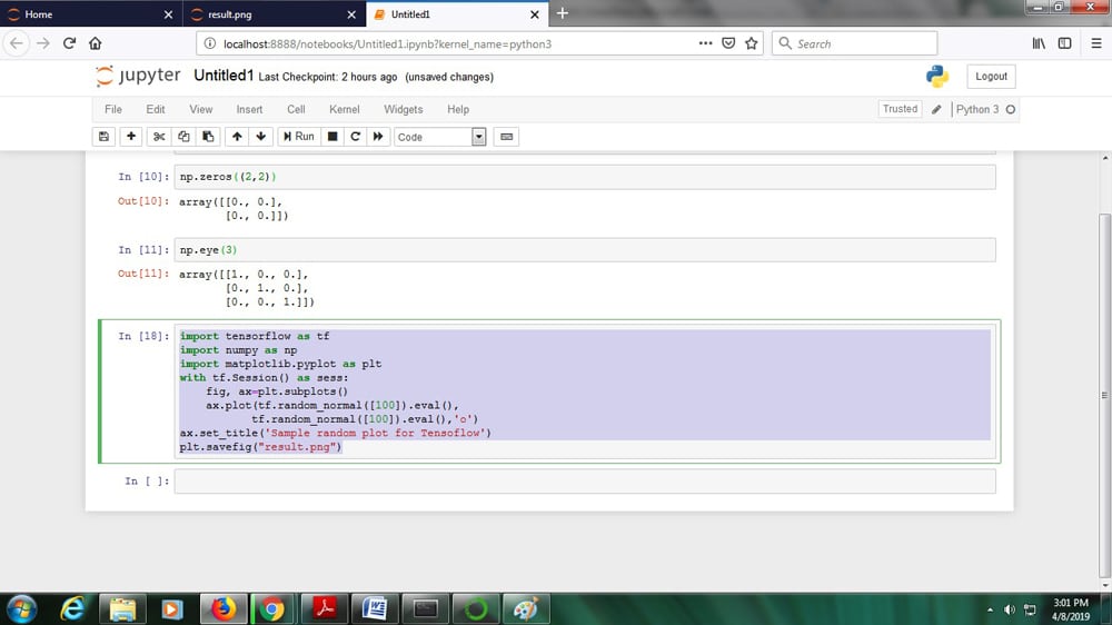
The TensorFlow library works under the alias of ‘tf’ and initialises the two variables as constants. It passes four numbers to the constant() function in Jupyter Notebook, resulting in an output.

Linear regression is the simple form of learning the parameters for any one-dimensional line. Let the data points be ‘x’ as one-dimensional and the class label ‘y’ generated by the linear equation:

y = mx+c

Here, ‘m’ and ‘c’ will be the learnable parameters that are calculated with the input. Now learn the parameters with TensorFlow by creating the artificial data set. To make this a bit hard, add a little bit of Gaussian noise to the data set, as follows:

y = mx+c+N(0,ε)

Introduction to classification

The creation of a machine learning model that is used to assign discrete labels to its particular input is called classification. Every discrete value is called a class and handles supervised learning algorithms with a discrete output. Here, the input is typically a feature vector and the output is a class. If there are only two class labels in the input (Yes/No, True/False, On/Off), it is called a binary classifier; otherwise, it is called a multiclass classifier.

Clustering data

Traversing files in TensorFlow: Unsupervised learning basically contains patterns of data sets. Clustering is mainly an unlabelled data set and helps to understand the groups of data with feature vectors. The data set is divided into a number of segments, where each and every point can be treated as a centroid, i.e., points belong to the particular group or cluster. Figure 5 shows the synthetic data set tensor code.

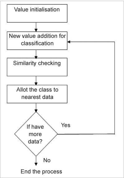
K-Means clustering on synthetic data sets: The flowchart for K-means clustering is given in Figure 6.

Machine learning empowers us to develop complex applications with extraordinary precision. TensorFlow helps to develop these applications.