Statistics is the discipline that involves the collection, organisation, display, analysis, interpretation and presentation of data. As data is today’s oil, its statistical analysis is very crucial. With LibreOffice Calc, one can perform complex statistical or engineering analyses to give different results based on the data provided.
The following operations can be performed with the help of LibreOffice Calc:
- Sampling
- Descriptive statistics
- Analysis of variance (ANOVA)
- Correlation
- Covariance
- Exponential smoothing
- Moving average
- Regression
- Paired t-test
- F-test
- Z-test
- Chi-square test
A brief description of each of these operations is given in this article.
Sampling
Sampling is the selection of a subset (a statistical sample) of individuals from within a statistical population to estimate the characteristics of the whole population.
Sampling is done row-wise, i.e., the sampled data picks the whole line of the source table and puts the result into a line of the target table.
Sampling methods
Random: Picks exact sample size lines of the source table randomly.
Sample size: This is the number of lines sampled from the source table.
Periodic: This method picks lines at a pace defined by Period.
Period: This is the number of lines to skip periodically when sampling.
To perform sampling, choose Data -> Statistics ->Sampling.
Sampling allows you to pick data from a source table/row and to fill a target table/row. The sampling can be random or periodical.
Data
Input: This refers to the range of the data to analyse.
Result: This refers to the top left cell of the range where the results are displayed.
In the input range, you have to specify the source of the data by selecting the columns. In ‘Results’ too, you have to specify the column name and row ID (e.g., $E$1 means column E and Row 1). This convention is followed for other methods also.
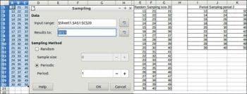
Next, you have to specify the sampling method. Once done, click ‘OK’ and you can see the desired output (Figure 1).
Descriptive statistics
Descriptive statistics is a summary that quantitatively describes or summarises features of a collection of information, and includes the process of using and analysing those statistics.
To perform descriptive statistics, choose Data -> Statistics -> Descriptive Statistics.
Fill a table in the spreadsheet with the main statistical properties of the data set.
Data
Input range: This refers to the range of the data to analyse.
Results to: This refers to the top left cell of the range where the results will be displayed.
Grouped by: Selects whether the input data has a columns or rows layout.
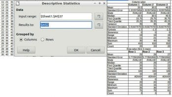
The example and output are shown in Figure 2.
Analysis Of Variance (ANOVA)
ANOVA is the acronym for Analysis Of Variance. It is a collection of statistical models and their associated estimation procedures (such as the ‘variation’ among and between groups) used to analyse the differences among the group means in a sample.
To perform ANOVA, choose Data > Statistics > Analysis of Variance (ANOVA).
Data
Input range: This refers to the range of the data to analyse.
Results to: This refers to the top left cell of the range where the results are displayed.
Grouped by: Selects whether the input data has a columns or rows layout.
Type: Selects if the analysis is for a single factor or for two-factor ANOVA.
Parameters
Alpha: This is the level of significance of the test.
Rows per sample: Defines how many rows a sample has.
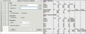
An example and results are shown in Figure 3.
Correlation
The correlation coefficient (a value between -1 and +1) refers to how strongly two variables are related to each other. You can use the CORREL function or the data statistics to find the correlation coefficient between two variables.
A correlation coefficient of +1 indicates a perfect positive correlation. A correlation coefficient of -1 indicates a perfect negative correlation. To perform correlation, choose Data > Statistics > Correlation.
Data
Input range: This refers to the range of the data to analyse.
Results to: This refers to the top left cell of the range where the results will be displayed.
Grouped by: Selects whether the input data has a columns or rows layout.
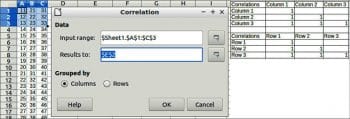
An example and results are shown in Figure 4.
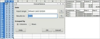
Covariance
This calculates the covariance of two sets of numeric data. The covariance is a measure of how much two random variables change together. To perform covariance, choose Data > Statistics > Covariance.
Data
Input range: Refers to the range of the data to analyse.
Results to: Refers to the top left cell of the range where the results will be displayed.
Grouped by: Selects whether the input data has a columns or rows layout.
An example and results are shown in Figure 5.
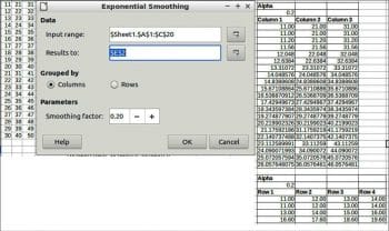
Exponential smoothing
Exponential smoothing is a filtering technique, which when applied to a data set, produces smooth results. It is employed in many domains such as the stock market, economics and in sampled measurements.
To perform exponential smoothing, choose Data > Statistics > Exponential smoothing.
Data
Input range: This refers to the range of the data to analyse.
Results to: This refers to the top left cell of the range where the results will be displayed.
Grouped by: Selects whether the input data has a columns or rows layout.
Parameters
Smoothing factor: A parameter between 0 and 1 represents the damping factor Alpha in the smoothing equation.
An example and results are given in Figure 6.
Moving average
This calculates the moving average of a time series. For the moving average, choose Data > Statistics > Moving average.
Data
Input range: This refers to the range of the data to analyse.
Results to: This refers to the top left cell of the range where the results will be displayed.
Grouped by: Selects whether the input data has a columns or rows layout.
Parameters
Interval: This is the number of samples used in the moving average calculation. An example and results are shown in Figure 7.
Regression
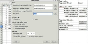
In statistical modelling, regression analysis is a set of statistical processes for estimating the relationships between a dependent variable (often called the ‘outcome variable’) and one or more independent variables (often called ‘predictors’, ‘covariates’ or ‘features’). The most common form of regression analysis is linear regression, in which the researcher finds the line (or a more complex linear function) that most closely fits the data according to a specific mathematical criterion. The other two types of regression that can be performed are logarithmic and power regression.
Here, two columns are required. Sample data is used here for imaginary time and temperature data.
An example and results are shown in Figure 8.
Paired t-test
The paired sample t-test, sometimes called the dependent sample t-test, is a statistical procedure used to determine whether the mean difference between two sets of observations is zero. In a paired sample t-test, each subject or entity is measured twice, resulting in pairs of observations.
To perform the paired t-test, choose Data > Statistics > Paired t-test.
Data
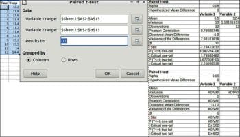
Variable 1 range: This refers to the range of the first data series to be analysed.
Variable 2 range: This refers to the range of the second data series to be analysed.
Results to: Refers to the top left cell of the range where the test will be displayed.
Grouped by: Selects whether the input data has a columns or rows layout.
An example and results are given in Figure 9.
F-test
This is any statistical test in which the test statistic has an F-distribution under the null hypothesis. It is most often used when comparing statistical models that have been fitted to a data set, in order to identify the model that best fits the population from which the data is sampled.
To perform the F-test, choose Data > Statistics > F-test.
Data
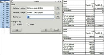
Variable 1 range: This refers to the range of the first data series to be analysed.
Variable 2 range: Refers to the range of the second data series to be analysed.
Results to: Refers to the top left cell of the range where the test will be displayed.
Grouped by: Selects whether the input data has a columns or rows layout.
An example and results are given in Figure 10.
Z-test
This is a statistical test used to determine whether two population means are different when the variances are known and the sample size is large.
To perform a Z-test, choose Data > Statistics > Z-test.
Data
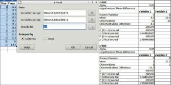
Variable 1 range: This refers to the range of the first data series to be analysed.
Variable 2 range: Refers to the range of the second data series to be analysed.
Results to: Refers to the top left cell of the range where the test will be displayed.
Grouped by: Selects whether the input data has a columns or rows layout.
An example and results are given in Figure 11.
Chi-square test
The phrase ‘a chi-squared test’, also written as a χ2 test, can be used as the description of any statistical hypothesis test where the sampling distribution of the test statistic is, under some circumstances, approximately (or what one hopes is approximately) a chi-squared distribution when the null hypothesis is true.
To perform the chi-square test, choose Data > Statistics > Chi-square test.
Data
Input range: This refers to the range of the data series to be analysed.
Results to: Refers to the top left cell of the range where the test will be displayed.
Grouped by: Selects whether the input data has a columns or rows layout.
An example and results are shown in Figure 12.
So, as indicated in brief here, twelve different kinds of statistical analyses, which help us to get some insight into our data sets, can be performed using Calc.


