Better late than never. If you missed the earlier discussions in this magazine related to deep learning tools and techniques, it’s time to refresh your learning.
Deep learning is not a new topic as such. It’s been around since 2014. However, the techniques and tools are evolving at a constant pace. A majority of them are free and open source software or FOSS. The investments are also considerable across organisations and geographies. As the practitioners say, we are in the prolonged summer phase of deep learning; so it’s never too late to jump into a beautiful paradigm of DL.
AI, ML and DL
Note: DL is the new kid on the block, a subset of ML and AI.
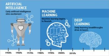
There’s always been some confusion about artificial intelligence (AI), machine learning (ML) and deep learning (DL). We often use these terms interchangeably. However, they actually are not the same. Artificial intelligence (AI) can be considered a superset of everything. AI can be viewed as automation of cognitive processes. Machine learning (ML), on the other hand, deals with the development of models out of training data sets. ML is a subset of AI. Deep learning (DL), in turn, is a subset of ML. It deals with the layering of models that have parameters, with a weight associated with each layer, and with continuously differentiable functions in a multi-dimensional space.
- Figure 1: The relationship between AI, ML and DL (Courtesy: Nikhil Gupta, Hackernoon)
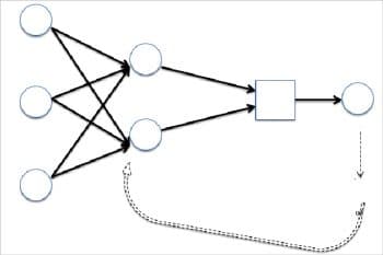
- Figure 2: Turning scrambled paper to unscrambled form through a network of nodes
Intuition and technique
Before getting into the techniques and tools of DL, let’s look at intuition first. Let us suppose that you have a crushed piece of paper in your hand that you are slowly and steadily opening out and flattening (or ‘unscrambling’) to its original form. DL is a similar process. When the initial data is available, it’s in a scrambled and tangled form. You can hardly get anything out of it. The DL process consists of a set of deep learning layers arranged as a network of nodes, called a neural network. Each layer has a parameter that we call the weight of the layer. There can be thousands of such layers and weights in a typical DL neural network. The DL process is all about opening out and flattening a crushed ball of paper. By passing the ‘scrambled’ data (in the form of an input tensor data structure) through the layer of the neural network, each layer is unscrambled a bit to finally flatten it out to a perfectly flat form. This final form often is in the shape of a vector, the 1D tensor.
Throughout the process, the weight of the layers is fine-tuned such that incremental unscrambling takes place. Of course, this process is iterative, and corrections over many iterations are collectively called epochs. Every time we measure the difference between what we want and what we get – the desired state minus the actual one. This gives us what is called the loss function. The sole purpose of the deep learning system is to minimise the loss function to attain the desired accuracy we want our DL model to achieve.
This always involves a feedback loop, where the loss function is minimised in each step by calibrating the weight. Technically speaking, the layer’s weight is adjusted a bit in the direction opposite to that of the gradient of continuous differentiation of the loss function with respect to the layer’s weight. This technique is called back propagation. Finally, the process converges at the end of the epoch and we have achieved our desired goal (often accuracy).
Note: Unscrambling a scrambled paper into a clear, flattened sheet through successive steps is the intuitive approach that DL is based on.
- Figure 3: Back propagation illustrated
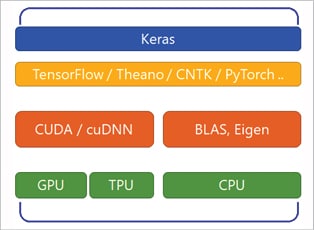
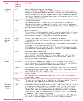
- Figure 4: Layers of a DL deployment taxonomy
Important definitions
Now, let’s get familiar with some of the DL related definitions we often encounter.
1. The model consists of a network of layers that have parameters (weights).
2. Layer: output = function
(weight, input)
3. Tensors: Data structures that represent input and output
4. Loss function: diff (expected output, actual output)
5. Differentiability: Gradient G = d (LossFunciont) d(Weight)
6. Gradient descent: Move layer’s weight in the opposite direction of G to reduce the loss function on every step.
7. Back propagation: Loopback through optimiser such that the loss function is minimised and runs through the gradient descent.
8. Evaluation: Measures the success (say, the accuracy of a prediction).
Taxonomy and tools
Before learning about the different tools involved in DL – platforms, languages, software – let us first find out more about the different layers in a typical DL deployment scenario.
Table 1 describes the FOSS tool taxonomy, from bottom to top, in the stack.
 Note: Keras is the best FOSS way to start with deep learning.
Keras installation
Keras can usually be deployed in many ways across platforms – Windows, Linux, Mac and even in the cloud (GCP, AWS). For practising DL programming using Keras, it is perfectly fine to have it running in the laptop with conventional CPUs on Windows as well. However, it is possible to book an EC2 GPU instance in AWS and get the benefit of a GPU. That way, one need not procure dedicated GPU hardware and can use the EC2 instance pay-as-you-go model. (However, for longer usage, the cloud may not necessarily be cost effective.)
Here we are going to describe the steps for the installation of Keras and associated dependencies in Ubuntu and Windows 10 using the underlying CPU of the laptop (no GPU needed).
Installation in Ubuntu
1. To install Python-2, use the following code:
sudo apt-get updatesudo apt-get install python-pip python |
2. In case you want to install Python-3 and want to make it the default Python, type:
sudo apt-get updatesudo apt-get install python3-pip python3alias python=python3alias pip=pip3 |
3. Install Python-specific scientific dependencies required for DL as follows.
a. For various Python math packages like NumPy, use:
sudo pip install matplotlibsudo pip install numpysudo pip install scipysudo pip install PyYAML |
b. To view the result (various graph viewers), type:
sudo pip install graphviz |
4. The code for installing Keras is:
sudo pip install keras |
The Keras config file can be found at ~/.keras/keras.json, which has information like backend: tensorflow.
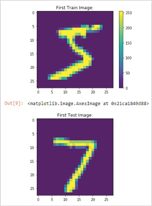
- Figure 5: MNIST data set digit output
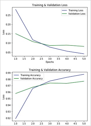
- Figure 6: MNIST data set training vs validation plotting
Installation in Windows 10
It is possible to install Keras in Windows 10 also, using Anaconda. The following steps need to be followed.
1. Download Anaconda https://www.anaconda.com/distribution/#download-section.
2. While installing Anaconda, you may optionally want to download the VSCode also as the preferred IDE for writing DL programs. However, you can use the Jupyter notebook as well, initially, for writing and running the program, piece-wise.
3. Next launch Anaconda Prompt from the Windows program launcher.
4. Next install Python-3.6:
conda install python=3.6 |
5. Create a conda environment:
conda env create -q -f environment.yml |
6. A typical environment.yml looks like:
name: practicechannels:- defaultsdependencies:- python=3.7.*- bz2file==0.98- cython==0.29.*- pip==19.1.*- numpy==1.16.*- jupyter==1.0.*- matplotlib==3.1.*- setuptools==41.0.*- scikit-learn==0.21.*- scipy==1.2.*- pandas==0.24.*- pillow==6.1.*- seaborn==0.9.*- h5py==2.9.*- pytest==5.0.*- twisted==19.2.*- tensorflow==1.13.* // For GPU it will be something like tensorflow-gpu==1.13.*- pip:- keras==2.2.* |
1. conda info –envs will show the practice as the environment.
2. conda activate practice
3. jupyter notebook
4. Launch http://localhost:8888/notebooks in your favourite browser.
A sample program using Keras
We are now going to look at the MNIST data set digit-detection problem using Jupyter Notebook.
To get an idea about what is inside the MNIST data set, use the following code:
import kerasfrom keras.datasets import mnistfrom keras import models, layersimport numpy as npimport matplotlib.pyplot as pltfrom keras.utils import to_categorical# Reading the mnist dataset which is 28X28 pixel of 70k integer (0-9) RBG scale images# Out of these 70K, I am using 60K to train my deep network, rest 10k will be used for validation/testing(train_images, train_labels), (test_images, test_labels) = mnist.load_data()print (train_images.shape);print (train_labels.shape);print (train_labels);# Lets see the images visually using MatPlotplt.figure()plt.title(‘First Train Image:’);plt.imshow(train_images[0]);plt.colorbar()plt.grid(False)plt.show();plt.title(‘First Test Image:’);plt.imshow(test_images[0]) |
The output is as shown in Figure 5.
Building the neural network
We have chosen a simple sequential network with two dense layers.
## Building the TensorFlow Network# As this is a categorical classification (multi-class, single label) problem, going with seq “Dense” sort of deep networksnetwork = models.Sequential();# First layer is downshaping the 28 x 28 image to a 512 tensor vector, relu is max(0, input)network.add(layers.Dense(512, activation=’relu’, input_shape=(28 * 28,)));# Now, add the last layer, downshaping the output of the previous layer to 10 (i.e. 0-9) ‘digits’.# Remember: The output of this layer is merely a probablistic distribution, hence “softmax”.network.add(layers.Dense(10, activation=’softmax’))## let’s see how DL network looks likenetwork.summary() |
The output is:
Instructions for updating:Co-locations handled automatically by placer.Model: “sequential_1”_______________________________________Layer (type) Output shape Param #=======================================dense_1 (Dense) (None, 512) 401920_______________________________________dense_2 (Dense) (None, 10) 5130=======================================Total params: 407,050Trainable params: 407,050Non-trainable params: 0_______________________________________________________ |
The compilation of the network can be done as follows:
# Let’s compile the network# Well: compile here means setting up the back propagation, defining the loss function and determining how the model is working## Optimiser is to reduce the loss function at every step, gradient descent, reducing d(loss_fn)/d (lthe ayer’s weight)# As it’s a categocial classification, picking up usual cat_crossent as loss method# How my network is converging? Lets measure ‘accuracy’network.compile(optimizer=’rmsprop’, loss=’categorical_crossentropy’, metrics=[‘accuracy’]); |
For data preparation, here’s the code snippet:
# Data preparation: To fit to my modeltrain_images = train_images.reshape((60000, 28 * 28))train_images = train_images.astype(‘float32’) / 255test_images = test_images.reshape((10000, 28 * 28))test_images = test_images.astype(‘float32’) / 255# Sort of encoding such that the value remains b/w [-1, to +1]train_labels = to_categorical(train_labels)test_labels = to_categorical(test_labels) |
Training can be done as follows:
# Now Training is done with 5 steps “epoch” on training data# Batch size typically power of 2, it’s the per batch processing in an epochvalidation_images = train_images[:10000]actual_train_images = train_images[10000:]validation_labels = train_labels[:10000]actual_train_labels = train_labels[10000:]history = network.fit(actual_train_images, actual_train_labels,epochs=5,batch_size=128,validation_data=(validation_images, validation_labels)) |
The output is:
Train on 50000 samples, validate on 10000 samplesEpoch 1/550000/50000[==================================] - 9s 178us/step - loss: 0.2801 - acc: 0.9191 - val_loss: 0.1498 - val_acc: 0.9578Epoch 2/550000/50000[=================================] - 5s 96us/step - loss: 0.1170 - acc: 0.9656 - val_loss: 0.1070 - val_acc: 0.9675Epoch 3/550000/50000[==================================] - 5s 100us/step - loss: 0.0773 - acc: 0.9770 - val_loss: 0.0858 - val_acc: 0.9739Epoch 4/550000/50000[=================================] - 5s 99us/step - loss: 0.0555 - acc: 0.9828 - val_loss: 0.0879 - val_acc: 0.9734Epoch 5/550000/50000[==================================] - 5s 94us/step - loss: 0.0414 - acc: 0.9874 - val_loss: 0.0812 - val_acc: 0.9767 |
Note: As you can see, the loss function (val_loss) is reducing at every step whereas the accuracy (val_acc) is increasing at every step. That’s the effectiveness of the training.
Here is the code snippet for training vs validation plotting:
# history object, output of fit methofhis_dict = history.historyprint (his_dict.keys())# loss plotting: Taining vs Validationloss_values = his_dict[‘loss’]val_loss_values = his_dict[‘val_loss’]epochs = range(1, len(his_dict[‘acc’]) + 1)plt.plot(epochs, loss_values, ‘b’, label=’Training Loss’)plt.plot(epochs, val_loss_values, ‘g’, label=’Validation Loss’)plt.title(‘Training & Validation Loss’)plt.xlabel(‘Epochs’)plt.ylabel(‘Loss’)plt.legend()plt.show()plt.clf() ## clear the plot# Accuracy plotting: Training vs Validationacc_values = his_dict[‘acc’]val_acc_values = his_dict[‘val_acc’]plt.plot(epochs, acc_values, ‘b’, label=’Training Accuracy’)plt.plot(epochs, val_acc_values, ‘g’, label=’Validation Accuracy’)plt.title(‘Training & Validation Accuracy’)plt.xlabel(‘Epochs’)plt.ylabel(‘Loss’)plt.legend()plt.show() |
The output is shown in Figure 6.
For testing over test data (10k samples), use the following code:
# Now it’s QA time! Test it over 10k samples.test_loss, test_acc = network.evaluate(test_images, test_labels)print(‘The accuracy I am expecting:’, test_acc); |
The output is:
10000/10000[====================================] - 1s 61us/stepThe accuracy I am expecting: 0.9752 |
The code for prediction is given below:
# Prediction sectionpredictions = network.predict(test_images);print (predictions.shape);print (‘Probablistic distribution of the first digit prediction: \n’ + str(predictions[0]));# See what we got?predicted_value = np.argmax(predictions[0]);print (‘Predicted pic: ‘ + str(predicted_value));print (‘Actual picture under test: ‘ + str(np.argmax(test_labels[0])));print (‘Bingo!’) |
The output is:
(10000, 10)Probablistic distribution of the first digit prediction:[2.10214646e-09 1.07541705e-10 1.82529277e-06 8.29521523e-057.31067290e-12 4.73346908e-08 1.90508078e-13 9.99913931e-012.09084714e-08 1.17789079e-06]Predicted pic: 7Actual picture under test: 7Bingo! |
Universal approach
The steps needed to attack and solve any DL problem are listed in Table 2.
- Figure 7: Google Colab GPU settings
- Figure 8: Google Colab Google Drive mount
Using Google Colab
Many of our laptops do not have GPUs, and are purely CPUs. So, what is the recourse? The answer is: Google Colab. It’s an attempt from Google to provide on-demand VMs with GPUs to run your tests. You can potentially mount your Google Drive as well to get the data from it. The steps given below will help you.
1. Log in to colab.research.google.com.
2. Look at File in the top menu.
3. You can write a new notebook or you can import an existing one.
4. You can go to the Edit > Notebook settings, where you can choose the hardware accelerator as the GPU. Refer to Figure 7.
5. You can even mount your Google Drive using the following code. Refer to Figure 8.
from google.colab import drivedrive.mount(‘/content/drive’)import tensorflow as tfprint (tf.test.gpu_device_name()) |
Deep learning has been evolving at a tremendous pace since the last couple of years. It is necessary to keep technically abreast with this emerging green field to stay relevant in the technical landscape. This article describes the taxonomy and various tools available at our disposal. While some are proprietary/commercial, there are plenty of FOSS tools around also. One of them is Keras. Familiarity with basic Python scripting is good enough to start with Keras. It abstracts the low-level languages (e.g., CUDA) and platforms (e.g., TensorFlow) beautifully to get a kickstart in this paradigm. It’s easy to install even on your laptops, and on Linux or Windows. A sample program of the MNIST data set digit detection has also been presented to give a glimpse of the anatomy of a DL program. This is just the beginning, and the road ahead is endless and enriching.
Note: The MNIST digit detection example mentioned in this article can be found in the following GitHub link: https://github.com/pradip-interra/MNIST-Digit-Detection

