Using PyTorch with Google Colab for Machine Learning

PyTorch is a free and open source, deep learning library developed by Facebook. Google Colab is a free online cloud based tool that lets you deploy deep learning models remotely on CPUs and GPUs. This article is an introduction to PyTorch, and will demonstrate its benefits by using a linear regression model to predict the value of a given piece of land, based on its size.

Machine learning and data science have emerged as some of the most sought after fields in the tech community. The number of use cases of machine learning is growing continuously — froma self-driving cars to smart home appliances. Open source deep learning libraries such as PyTorch and TensorFlow have been gaining a lot of steam. Within just three years of its initial release in 2016, PyTorch has become very popular with companies like Apple, Verizon, NVIDIA and Uber, and is being used in their deep learning projects.

PyTorch
The initial purpose behind creating PyTorch was to replace the use of Numpy arrays with the more sophisticated tensors, which are similar, except that the latter perform much better with GPUs. It has now become a market leader and competitor to Google’s TensorFlow library.

The main component of PyTorch is the Torch library, written in the Lua scripting language, which provides the facility to create n-dimensional tensors (arrays) that support all the basic operations such as slicing, indexing and transposing. Additionally, it supports operations such as max, min and sum, and the more advanced tensor operations like vector multiplication. Development on the Torch library stopped in 2018. However, the PyTorch library is in active development by Facebook. The latest version of PyTorch was released in October 2019.

What is Google Colab?
The Google Colab (short for Colaboratory) is a research project launched by Google. Its intended purpose is to make the life of developers easier by giving them the facility to remotely deploy deep learning models on the CPUs and GPUs being offered in the form of virtual machines. It is based on the powerful open source technology, Jupyter, with which you can create an Ipython notebook. The Ipython notebook not only gives you the ability to write code, but to also tell a story through it, in an illustrated manner. You can execute code, create beautiful and vivid visualisations of your data, and write about each step you make in plain text or HTML. This makes your code look less like a simple program and more like a textbook, with step-by-step explanations and visualisations of what the code does.

One of the major benefits of Google Colab is that it supports development in both Python2 and Python3. Currently, it does not support the R programming language. Google Colab supports the installation and import of all the major machine learning libraries such as Numpy, TensorFlow, PyTorch, Scikitlearn, Matplotlib, Seaborn, Pandas, etc.

You can save the Ipython notebooks that you create straight to your Google Drive, thus making sure your data is always available on the cloud. Another major benefit is the ease with which you can share your notebooks with anyone online. You can collaborate with your peers remotely on Google Colab by setting the appropriate permissions for others editing your notebook.

Setting up Google Colab
Creating a notebook on Google Colab is super easy. All you need is a Google account. Just follow the steps listed below.

1. Open your Web browser and go to drive.google.com.
2. Log in using your Google account.
3. On your Drive, click New → Folder.
4. You can name your folder whatever you like. For the purpose of this demonstration, let’s call it learn-pytorch.
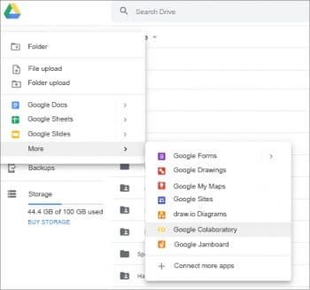
5. Go to the folder you just created and then click New → More → Google Colaboratory as shown in Figure 1.
6. This will take you to your Google Colab notebook. On the top left, an automatically generated name of the file will be displayed, which could be something like Untitled0.ipynb. The extension .ipynb stands for the Ipython notebook. Click on the name and rename it linear regression using pytorch.ipynb.
7. On the left side of the top panel, below the main menu, you will see two buttons, ‘+ code’ and ‘+ text’, which you can use to create code or text snippets based on your requirements.
8. On the right side of the panel, you will be able to find the options to view the RAM and disk space allotted to you, as well as how much of it you have already used.
9. In order to test that everything is working properly, simply write the following code in the automatically generated first code cell:

   print(‘Hello World’)

10. Now press the Shift + Return key to execute the code or click the little Play sign at the beginning of the cell to execute the command. Your expected output should be displayed below the code as ‘Hello World’.

And that’s it; we are done with the basic setup! Let us start executing our code.

Deploying the model
The first thing is to check if PyTorch is already installed and if not, we need to install it. We will do this by running the following piece of code:

!pip3installtorch

Next, let us import the following libraries for the code execution:

import numpy as np
import pandas as pd
import matplotlib.pyplot as plt
import torch
from torch.autograd import Variable

In order to simplify things for the purpose of this demonstration, let us create some dummy data of the land’s dimensions and its corresponding price with 20 entries. If you would like to directly read this data in the form of a .csv file, you can download it from the URL given at the end of this article.

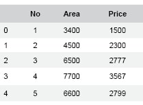
#Create the training data
no = [1,2,3,4,5,6,7,8,9,10,11,12,13,14,15,16,17,18,19,20]
area = [3400,4500,6500,7700,6600,3500,4300,3700,8700,9000,9100,9200,8200,8800,8400,8300,7900,7400,7100,6400]
price = [1500,2300,2777,3567,2799,1633,2111,1700,4333,4500,4551,4560,4200,4304,4000,4230,3700,3300,3000,2600]
data = pd.DataFrame({‘No’:no,’Area’:area,’Price’:price})

data.head()

The data.head() method will help us see the first five rows of our data frame, as shown in Figure 2. Now, let us create a sample test data to test our model.

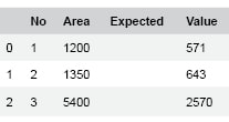
#create the test data
index = [1,2,3]
area_size = [1200, 1350, 5400]
area_value = [571, 643, 2570]
test_data = pd.DataFrame({‘No’:index, ‘Area’: area_size, ‘Expected Value’: area_value})

test_data.head()

Figure 3 shows the visual of the test data. The next step is to convert the data into a proper Numpy array, which we can then use to train our model.

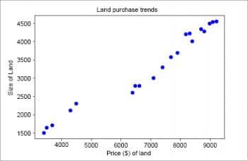
#convert the data into a numpy array
data = np.array(data,dtype=np.float32)
x_train = data[: ,1:2]
y_train = data[: ,2:3]

test_data = np.array(test_data,dtype=np.float32)
x_test = test_data[:,1:2]
y_test = test_data[:, 2:3]

#visualize the data using a scatter plot
plt.plot(x_train, y_train, ‘bo’)
plt.xlabel(“Price ($) of land”)
plt.ylabel(“Size of Land”)
plt.title(“Land purchase trends”)
plt

Figure 4 shows the visualisation of the data. From the scatter plot, we can clearly see a positive correlation in the data, i.e., as the size of the land increases, so does its price. Hence, we can draw a line across this data to derive predictions of what the value of a given piece of land might be, given its size.

We will define a linear regression class with the help of the torch.nn module, which has a linear model available that takes two parameters — input size and the output size. Additionally, we will also define a forward class method inside our function to derive the output of the model.

class LinReg(torch.nn.Module):
def __init__(self, input_size, output_size):
super(LinReg, self).__init__()
self.linear = torch.nn.Linear(input_size, output_size)

def forward(self, x):
out = self.linear(x)
return out

We can instantiate the model using the following code:

#define input/output dimensions, learning rate and the no. of epochs to run
input_dimension = 1
output_dimension = 1
learn_rate =0.000000001
epochs = 100

model = LinReg(input_dimension, output_dimension)
##### For GPU #######
if torch.cuda.is_available():
model.cuda()

Next, we will initialise the loss (Mean Squared Error) and optimisation (Stochastic Gradient Descent) functions that we’ll use in the training of this model:

criterion = torch.nn.MSELoss()
optimizer = torch.optim.SGD(model.parameters(), lr=learn_rate)

After completing all the initialisations, we can now begin to train our model. The following code is for training the model:

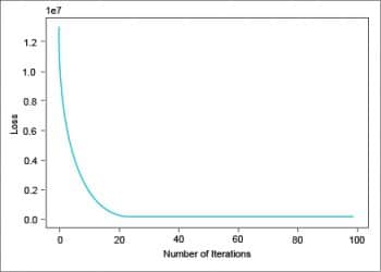
losses=[]
for epoch in range(epochs):
# Convert the inputs and labels to Variables
if torch.cuda.is_available():
inputs = Variable(torch.from_numpy(x_train).cuda())
labels = Variable(torch.from_numpy(y_train).cuda())
else:
inputs = Variable(torch.from_numpy(x_train))
labels = Variable(torch.from_numpy(y_train))

# Clear gradient buffers in order to avoid cumulation of gradients
optimizer.zero_grad()

# get output from the model
outputs = model(inputs)

# get the loss for the predicted output
loss = criterion(outputs, labels)
# get the gradients
loss.backward()
# update parameters
optimizer.step()
losses.append(loss.data)
if(epoch%10==0):
print(‘epoch {}, loss {}’.format(epoch, loss.data))
plt.plot(range(epochs),losses)
plt.xlabel(“Number of Iterations”)
plt.ylabel(“Loss”)
plt

The above code will give you a visualisation of the performance of the loss function over 100 epochs. Figure 5 shows that the loss rate is steadily decreasing and is at its lowest near the 100th iteration.
Now that our linear regression model is trained, let’s test it. We will first use our model to predict the values of the training data itself, and visualise the line to see how accurately we are able to predict the values.

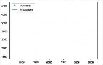
with torch.no_grad():
if torch.cuda.is_available():
predicted = model(Variable(torch.from_numpy(x_train).cuda())).cpu().data.numpy()
else:
predicted = model(Variable(torch.from_numpy(x_train))).data.numpy()
print(“predicted=”,predicted)

plt.clf()
plt.plot(x_train, y_train, ‘go’, label=’True data’, alpha=0.5)
plt.plot(x_train, predicted, ‘-’, label=’Predictions’, alpha=0.5)
plt.legend(loc=’best’)
plt.show()

Figure 6 shows the linear model predicting the training data very accurately. Now let us try the same thing using the test data we created earlier:

with torch.no_grad(): # we don’t need gradients in the testing phase
if torch.cuda.is_available():
predicted = model(Variable(torch.from_numpy(x_test).cuda())).cpu().data.numpy()
else:
predicted = model(Variable(torch.from_numpy(x_test))).data.numpy()
print(“predicted=”,predicted)

plt.clf()
plt.plot(x_test, y_test, ‘go’, label=’Test Data’, alpha=0.5)
plt.plot(x_test, predicted, ‘-’, label=’Predictions’, alpha=0.5)
plt.legend(loc=’best’)
plt.show()

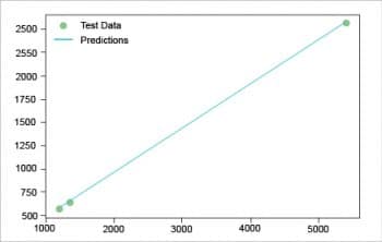
Figure 7 shows that we have accurately predicted the values of the test data as well. The linear regression model has been successfully executed. You can find all the source code resources used in this article at https://github.com/shah78677/PyTorch-Experiments.