A basic knowledge of SQL and its query language is essential for any aspiring data analyst and data scientist. This article discusses SQL and its data analysis features.
Structured Query Language (SQL) is a must for a data analyst or data scientist. SQL provides the basic storage and retrieval platform for organisations working with data. It provides rich data retrieval and report generation facilities, along with numerous data storage and security features. Though it is a complex multi-layered system, it is still simple and easy to understand. This is why data analysts are using SQL to understand and explore data before moving to higher levels of analysis and visualisation.
What is SQL and why is it so popular?
SQL is a relational database system and is used to create, store and process data. But for a data analyst, it is better to compare SQL with a spreadsheet, particularly with Microsoft’s Excel. Both SQL and Excel are simple and robust for data storage, but there are differences when it comes to handling them. Excel is basically a graphical user interface and performs data visualisation in a very simple way. It provides a shallow data analysis platform (only one workbook) with the graphical visualisation facility. Moreover, it is not meant for high volumes of data. SQL, on the other hand, is very rich in data analysis, especially in report generation. It supports very complex analysis (queries) combining multiple tables and databases. SQL also supports analysis in different forms, like interactive and stored (in the form of stored procedures and virtual tables (VIEW)) queries.
Excel is suitable for smaller data sets, and becomes slow and inefficient when the data is filtered with complex formulas. This performance degradation is quite high for a data sheet with only a few thousand rows. In SQL, even 10 million rows can be processed fairly quickly.
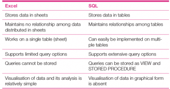
Though it has many advantages over Excel, SQL is still used only for simple tasks like aggregating data, joining data sets, and performing complex statistical and mathematical computations.
SQL is also rich in data analysis features. A discussion covering all of them in this limited space is not feasible. In this article, I will explore some of the most useful data analysis features of SQL. Its other important features and its data analysis functionalities will be discussed later.
Data processing
Typically, data processing means operating on numerical and character strings. SQL supports both and provides various operators for them. Among different arithmetic, logical and relational operators, IS NUL, BETWEEN, IN and EXISTS are the most important and provide powerful searching options that are frequently used for data analysis tasks.
Resources
The analysis has been done on Northwind and world.sql RDBMS. These are available in the Google archives https://code.google.com/archive/p/northwindextended/downloads and https://dev.mysql.com/doc/index-other.html. Readers can download the data and experiment with it in their own way.
Data analysis
Since SQL is advantageous for storage and security reasons, it is widely used for storage, the aggregation of data, joining of tables, etc. Here I will discuss a few data analysis features of SQL.
Grouping
Aggregation of field values on different categories of a given field is a good option for category-wise data analysis and visualisation. For example, in a world database, to add the population of all cities of a country, we can group the city table on the basis of the country’s identification code.
use world
select a.CountryCode, sum(a.Population)
from city as a
group by a.CountryCode
order by a.CountryCode
limit 5
This grouping can be made selective by using the HAVING clause. For instance, if the data analysis requires the total population figures of a few selected countries only, we can write the code using IN and BETWEEN as follows:
select a.CountryCode, sum(a.Population) as Population
from city as a
group by a.CountryCode
having a.CountryCode in ("ABW","AFG","ALB")
order by a.CountryCode
limit 5
The analysis report of the above query is as follows: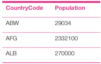
select a.CountryCode, sum(a.Population) as Population
from city as a
group by a.CountryCode
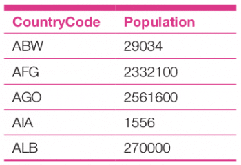
having a.CountryCode between “ABW” and “ALB”
order by a.CountryCode
limit 5
The analysis report is as follows:
 Joining tables
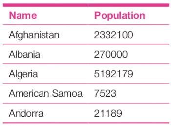
Joining multiple tables using their Cartesian product is an important feature of SQL. It provides the true benefit of a relational database system. Combined virtual table, of related data, mapped through the key fields, is frequently used in data analysis. For example, to replace the country code with the actual name we can join the city table with the country table on the basis of the country code, and then replace it with the actual name in the report.
select b.name,sum(a.Population) as Population
from city as a
join country as b on b.Code=a.CountryCode
group by a.CountryCode
order by b.name
The analysis report is as follows:
 Self-join
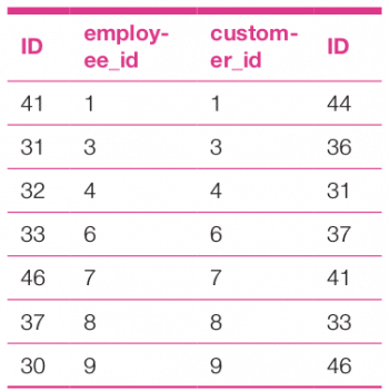
Self-join is used to analyse a table with respect to itself. It has several utilities. Here I have used this concept to identify those employees who have ordered some products by joining the orders table with itself on the basis of employee_id and customer_id:
use northwind;
select
a.id,a.employee_id,b.customer_id,b.id
from orders as a, orders as b
where a.employee_id = b.customer_id
group by a.employee_id
The analysis report of the self-join query is as follows:
The same idea can be used to analyse the table orders to find out those employees who have ordered on the same date.
use northwind;
select
a.id,a.employee_id,b.customer_id,b.id,a.order_date,b.order_date
from orders as a, orders as b
where a.order_date = b.order_date and a.employee_id = b.customer_id
group by a.employee_id
The analysis report of the above query is as follows:
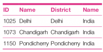
 In a similar case, if we consider the world database, then to find all the cities in India for which the name of the city and the district are the same, one can try the following query:
use world;
select distinct
a.ID,a.Name,b.District,c.Name
from city as a, city as b
inner join country as c on c.Code=b.CountryCode
where a.Name = b.District and c.Name=’India’
The analysis report shows the following:
 Union
Union
From the analysis point of view, the union of tables is a useful feature of SQL. It provides a combination of more than one table on the basis of common field values. This set union functionality has several uses. One of the most practical uses may be analysing the current transaction table with archive tables. Here, to illustrate the use of union, I have considered the overall frequency distribution of job categories among the employees and customers in the Northwind database.
select a.job_title,count(a.job_title) Frequency
from (select * from customers
union
select * from employees) as a
group by a.job_title
order by a.job_title
Intersection
Intersect is used to find common records from the participating tables. For instance, to find all the common records from both the customer and employee tables, one can use the following code:
select concat_ws(“ “,c.first_name,c.last_name) as name, c.city
from
(select a.city,a.last_name,a.first_name from customers as a
intersect
select b.city,b.last_name,b.first_name from employees as b) as c
Subquery
Subquery is an essential tool for data analysis. It provides a virtual table during execution of the existing query. In the above union and intersect queries, the subquery feature is used to provide union and intersection of customers and employees to the main query.
Though SQL supports stored queries like VIEW and STORED PROCEDURE, it suffers from a lack of flexibility. As it is embedded within an RDBMS, it cannot exhibit all the flexibility of a programming language and is also not safe. In addition to this, since its data visualisation capacity is limited, very often it becomes essential to port data to another platform for further analysis and visualisation. R and Python are good for data analysis, while SQL is commonly used as an embedded program from these two languages. This gives additional programming capabilities to SQL, and makes the data analysis and visualisation more versatile.


