Version 2.0 of TensorFlow is focused on simplicity and ease of use. It has been strengthened with updates like eager execution and intuitive higher level APIs accompanied by flexible model building. It is platform agnostic, and makes APIs more consistent, while removing those that are redundant.
Machine learning and artificial intelligence are experiencing a revolution these days, primarily due to three major factors. The first is the increased computing power available within small form factors such as GPUs, NPUs and TPUs. The second is the breakthrough in machine learning algorithms. State-of-art algorithms and hence models are available to infer faster. Finally, huge amounts of labelled data is essential for deep learning models to perform better, and this is now available.
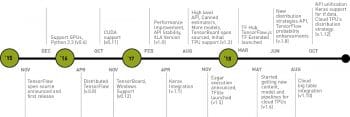
TensorFlow is an open source AI framework from Google which arms researchers and developers with the right tools to build novel models. It was made open source in 2015 and, in the past few years, has evolved with various enhancements covering operator support, programming languages, hardware support, data sets, official models, and distributed training and deployment strategies.
TensorFlow 2.0 was released recently at the TensorFlow Developer Summit. It has major changes across the stack, some of which will be discussed from the developers’ point of view.
TensorFlow 2.0 is primarily focused on the ease-of-use, power and scalability aspects. Ease is ensured in terms of simplified APIs, Keras being the main high level API interface; eager execution is available by default. Version 2.0 is powerful in the sense of being flexible and running much faster than earlier, with more optimisation. Finally, it is more scalable since it can be deployed on high-end distributed environments as well as on small edge devices.
This new release streamlines the various components involved, from data preparation all the way up to deployment on various targets. High speed data processing pipelines are offered by tf.data, high level APIs are offered by tf.keras, and there are simplified APIs to access various distribution strategies on targets like the CPU, GPU and TPU. TensorFlow 2.0 offers a unique packaging format called SavedModel that can be deployed over the cloud through a TensorFlow Serving. Edge devices can be deployed through TensorFlow Lite, and Web applications through the newly introduced TensorFlow.js and various other language bindings that are also available.

TensorFlow.js was announced at the developer summit with off-the-shelf pretrained models for the browser, node, desktop and mobile native applications. The inclusion of Swift was also announced. Looking at some of the performance improvements since last year, the latest release claims a training speedup of 1.8x on NVIDIA Tesla V100, a 1.6x training speedup on Google Cloud TPUv2 and a 3.3.x inference speedup on Intel Skylake.
Upgrade to 2.0
The new release offers a utility tf_upgrade_v2 to convert a 1.x Python application script to a 2.0 compatible script. It does most of the job in converting the 1.x deprecated API to a newer compatibility API. An example of the same can be seen below:
test-pc:~$cat test-infer-v1.py

# Tensorflow imports
import tensorflow as tf

save_path = ‘checkpoints/dev’
with tf.gfile.FastGFile(“./trained-graph.pb”, ‘rb’) as f:
graph_def = tf.GraphDef()
graph_def.ParseFromString(f.read())
tf.import_graph_def(graph_def, name=’’)

with tf.Session(graph=tf.get_default_graph()) as sess:
input_data = sess.graph.get_tensor_by_name(“DecodeJPGInput:0”)
output_data = sess.graph.get_tensor_by_name(“final_result:0”)

image = ‘elephant-299.jpg’
if not tf.gfile.Exists(image):
tf.logging.fatal(‘File does not exist %s’, image)
image_data = tf.gfile.FastGFile(image, ‘rb’).read()

result = sess.run(output_data, {‘DecodeJPGInput:0’: image_data})
print(result)

test-pc:~$ tf_upgrade_v2 --infile test-infer-v1.py --outfile test-infer-v2.py

INFO line 5:5: Renamed ‘tf.gfile.FastGFile’ to ‘tf.compat.v1.gfile.FastGFile’
INFO line 6:16: Renamed ‘tf.GraphDef’ to ‘tf.compat.v1.GraphDef’
INFO line 10:9: Renamed ‘tf.Session’ to ‘tf.compat.v1.Session’
INFO line 10:26: Renamed ‘tf.get_default_graph’ to ‘tf.compat.v1.get_default_graph’
INFO line 15:15: Renamed ‘tf.gfile.Exists’ to ‘tf.io.gfile.exists’
INFO line 16:12: Renamed ‘tf.logging.fatal’ to ‘tf.compat.v1.logging.fatal’
INFO line 17:21: Renamed ‘tf.gfile.FastGFile’ to ‘tf.compat.v1.gfile.FastGFile’
TensorFlow 2.0 Upgrade Script
-----------------------------
Converted 1 files
Detected 0 issues that require attention
-------------------------------------------------------------
Make sure to read the detailed log ‘report.txt’

test-pc:~$ cat test-infer-v2.py

# Tensorflow imports
import tensorflow as tf

save_path = ‘checkpoints/dev’
with tf.compat.v1.gfile.FastGFile(“./trained-graph.pb”, ‘rb’) as f:
graph_def = tf.compat.v1.GraphDef()
graph_def.ParseFromString(f.read())
tf.import_graph_def(graph_def, name=’’)

with tf.compat.v1.Session(graph=tf.compat.v1.get_default_graph()) as sess:
input_data = sess.graph.get_tensor_by_name(“DecodeJPGInput:0”)
output_data = sess.graph.get_tensor_by_name(“final_result:0”)

image = ‘elephant-299.jpg’
if not tf.io.gfile.exists(image):
tf.compat.v1.logging.fatal(‘File does not exist %s’, image)
image_data = tf.compat.v1.gfile.FastGFile(image, ‘rb’).read()

result = sess.run(output_data, {‘DecodeJPGInput:0’: image_data})
print(result)
As we can see here, the tf_upgrade_v2 utility converts all the deprecated APIs to compatible v1 APIs, to make them work with 2.0.
Eager execution: Eager execution allows real-time evaluation of Tensors without calling session.run. A major advantage with eager execution is that we can print the Tensor values any time for debugging.
With TensorFlow 1.x, the code is:
test-pc:~$python3
Python 3.6.7 (default, Oct 22 2018, 11:32:17)
[GCC 8.2.0] on linux
Type “help”, “copyright”, “credits” or “license” for more information.
>>> import tensorflow as tf
>>> print(tf.__version__)
1.14.0
>>> tf.add(2,3)
<tf.Tensor ‘Add:0’ shape=() dtype=int32>
TensorFlow 2.0, on the other hand, evaluates the result that we call the API:
test-pc:~$python3
Python 3.6.7 (default, Oct 22 2018, 11:32:17)
[GCC 8.2.0] on linux
Type “help”, “copyright”, “credits” or “license” for more information.
>>> import tensorflow as tf
>>> print(tf.__version__)
2.0.0-beta1
>>> tf.add(2,3)
<tf.Tensor: id=2, shape=(), dtype=int32, numpy=5>
In v1.x, the resulting Tensor doesn’t display the value and we need to execute the graph under a session to get the value, but in v2.0 the values are implicitly computed and available for debugging.
Keras
Keras (tf.keras) is now the official high level API. It has been enhanced with many compatible low level APIs. The redundancy across Keras and TensorFlow is removed, and most of the APIs are now available with Keras. The low level operators are still accessible through tf.raw_ops.
We can now save the Keras model directly as a Tensorflow SavedModel, as shown below:
# Save Model to SavedModel
saved_model_path = tf.keras.experimental.export_saved_model(model, ‘/path/to/model’)

# Load the SavedModel
new_model = tf.keras.experimental.load_from_saved_model(saved_model_path)

# new_model is now keras Model object.
new_model.summary()
Earlier, APIs related to various layers, optimisers, metrics and loss functions were distributed across Keras and native TensorFlow. Latest enhancements unify them as tf.keras.optimizer.*, tf.keras.metrics.*, tf.keras.losses.* and tf.keras.layers.*.
The RNN layers are now much more simplified compared to v 1.x.
With TensorFlow 1.x, the commands given are:
if tf.test.is_gpu_available():
model.add(tf.keras.layers.CudnnLSTM(32))
else
model.add(tf.keras.layers.LSTM(32))
With TensorFlow 2.0, the commands given are:
# This will use Cudnn kernel when the GPU is available.
model.add(tf.keras.layer.LSTM(32))
TensorBoard integration is now a simple call back, as shown below:
tb_callbaclk = tf.keras.callbacks.TensorBoard(log_dir=log_dir)

model.fit(
x_train, y_train, epocha=5,
validation_data = [x_test, y_test],
Callbacks = [tb_callbacks])
With this simple call back addition, TensorBoard is up on the browser to look for all the statistics in real-time.
Keras offers unified distribution strategies, and a few lines of code can enable the required strategy as shown below:
strategy = tf.distribute.MirroredStrategy()

with strategy.scope()
model = tf.keras.models.Sequential([
tf.keras.layers.Dense(64, input_shape=[10]),
tf.keras.layers.Dense(64, activation=’relu’),
tf.keras.layers.Dense(10, activation=’softmax’)])

model.compile(optimizer=’adam’,
loss=’categorical_crossentropy’,
metrics=[‘accuracy’])
As shown above, the model definition under the desired scope is all we need to apply the desired strategy. Very soon, there will be support for multi-node synchronous and TPU strategy, and later, for parameter server strategy.

TensorFlow function
Function is a major upgrade that impacts the way we write TensorFlow applications. The new version introduces tf.function, which simplifies the applications and makes it very close to writing a normal Python application.
A sample tf.function definition looks like what’s shown in the code snippet below. Here the tf.function declaration makes the user define a function as a TensorFlow operator, and all optimisation is applied automatically. Also, the function is faster than eager execution. APIs like tf.control_dependencies, tf.global_variable_initializer, and tf.cond, tf.while_loop are no longer needed with tf.function. The user defined functions are polymorphic by default, i.e., we may pass mixed type tensors.
test-pc:~$ cat tf-test.py
import tensorflow as tf

print(tf.__version__)

@tf.function
def add(a, b):
return (a+b)

print(add(tf.ones([2,2]), tf.ones([2,2])))

test-pc:~$ python3 tf-test.py
2.0.0-beta1
tf.Tensor(
[[2. 2.]
[2. 2.]], shape=(2, 2), dtype=float32)
Here is another example to demonstrate automatic control flows and Autograph in action. Autograph automatically converts the conditions, while it loops Python to TensorFlow operators.
test-pc:~$ cat tf-test-control.py
import tensorflow as tf

print(tf.__version__)

@tf.function
def f(x):
while tf.reduce_sum(x) > 1:
x = tf.tanh(x)
return x

print(f(tf.random.uniform([10])))

test-pc:~$ python3 tf-test-control.py

2.0.0-beta1
tf.Tensor(
[0.10785562 0.11102211 0.11347286 0.11239681 0.03989326 0.10335539
0.11030331 0.1135259 0.11357211 0.07324989], shape=(10,), dtype=float32)
We can see Autograph in action with the following API over the function.
print(tf.autograph.to_code(f)) # f is the function name
TensorFlow Lite
The latest advancements in edge devices add neural network accelerators. Google has released EdgeTPU, Intel has the edge inference platform Movidius, Huawei mobile devices have the Kirin based NPU, Qualcomm has come up with NPE SDK to accelerate on the Snapdragon chipsets using Hexagon power and, recently, Samsung released Exynos 9 with NPU. An edge device optimised framework is necessary to support these hardware ecosystems.
Unlike TensorFlow, which is widely used in high power-consuming server infrastructure, edge devices are challenging in terms of reduced computing power, limited memory and battery constraints. TensorFlow Lite is aimed at bringing in TensorFlow models directly onto the edge with minimal effort. The TF Lite model format is different from TensorFlow. A TF Lite converter is available to convert a TensorFlow SavedBundle to a TF Lite model.
Though TensorFlow Lite is evolving, there are limitations too, such as in the number of operations supported, and the unsupported semantics like control-flows and RNNs. In its early days, TF Lite used a TOCO converter and there were a few challenges for the developer community. A brand new 2.0 converter is planned to be released soon. There are claims that using TF Lite results in huge improvements across the CPU, GPU and TPU.
TF Lite introduces delegates to accelerate parts of the graph on an accelerator. We may choose a specific delegate for a specific sub-graph, if needed.
#import “tensorflow/lite/delegates/gpu/metal_delegate.h”

// Initialize interpreter with GPU delegate
std::unique_ptr<Interpreter> interpreter;
InterpreterBuilder(*model, resolver)(&interpreter);
auto* delegate = NewGpuDelegate(nullptr); // default config
if (interpreter->ModifyGraphWithDelegate(delegate) != kTfLiteOk) return false;

// Run inference
while (true) {
WriteToInputTensor(interpreter->typed_input_tensor<float>(0));
if (interpreter->Invoke() != kTfLiteOk) return false;
ReadFromOutputTensor(interpreter->typed_output_tensor<float>(0));
}

// Clean up
interpreter = nullptr;
DeleteGpuDelegate(delegate);
As shown above, we can choose GPUDelegate, and modify the graph with the respective kernel’s runtime. TF Lite is going to support the Android NNAPI delegate, in order to support all the hardware that is supported by NNAPI. For edge devices, CPU optimisation is also important, as not all edge devices are equipped with accelerators; hence, there is a plan to support further optimisations for ARM and x86.
Optimisations based on quantisation and pruning are evolving to reduce the size and processing demands of models. Quantisation generally can reduce model size by 4x (i.e., 32-bit to 8-bit). Models with more convolution layers may get faster by 10 to 50 per cent on the CPU. Fully connected and RNN layers may speed up operation by 3x.
TF Lite now supports post-training quantisation, which reduces the size along with compute demands greatly. TensorFlow 2.0 offers simplified APIs to build models with quantisation and by pruning optimisations.
A normal dense layer without quantisation looks like what follows:
tf.keras.layers.Dense(512, activation=’relu’)
Whereas a quality dense layer looks like what’s shown below:
quantize.Quantize(tf.keras.layers.Dense(512, activation=’relu’))
Pruning is a technique used to drop connections that are ineffective. In general, ‘dense’ layers contain lots of connections which don’t influence the output. Such connections can be dropped by making the weight zero. Tensors with lots of zeros may be represented as ‘sparse’ and can be compressed. Also, the number of operations in a sparse tensor is less.
Building a layer with prune is as simple as using the following command:
prune.Prune(tf.keras.layers.Dense(512, activation=’relu’))
In a pipeline, there is Keras based quantised training and Keras based connection pruning. These optimisations may push TF Lite further ahead of the competition, with regard to other frameworks.
Coral
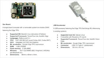
Coral is a new platform for creating products with on-device ML acceleration. The first product here features Google’s Edge TPU in SBC and USB form factors. TensorFlow Lite is officially supported on this platform, with the salient features being very fast inference speed, privacy and no reliance on network connection.
More details related to hardware specifications, pricing, and a getting started guide can be found at https://coral.withgoogle.com.
With these advances as well as a wider ecosystem, it’s very evident that TensorFlow may become the leading framework for artificial intelligence and machine learning, similar to how Android evolved in the mobile world.


