


Deep learning is impacting and revolutionising the tech industry. Many applications used on a day-to-day basis have been built incorporating deep learning. This article explains how the popular TensorFlow framework can be used to build a deep learning model.
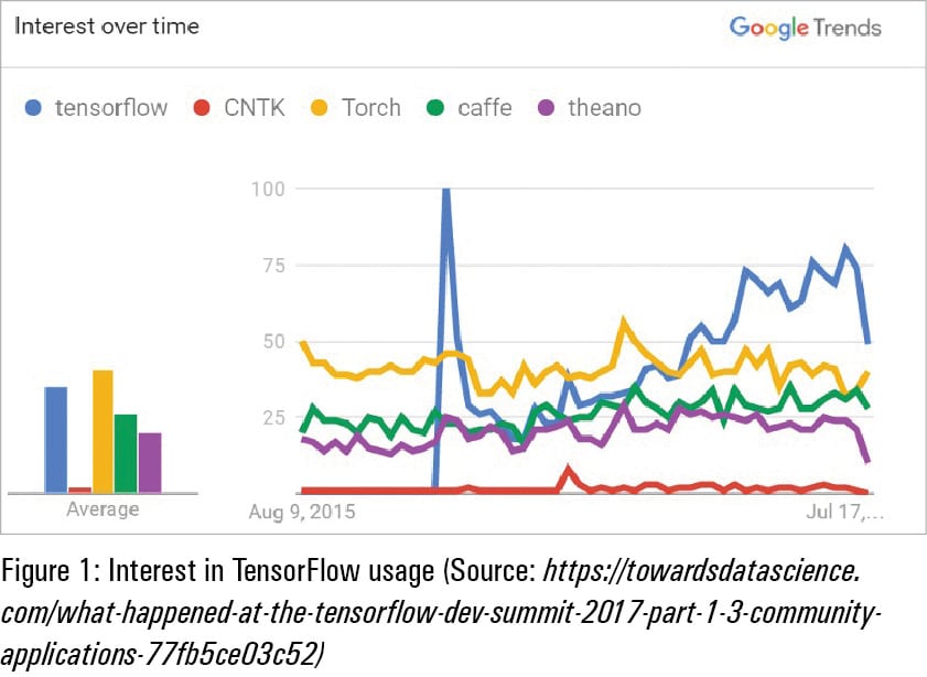
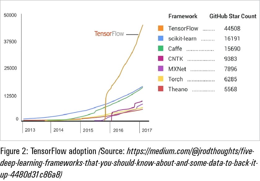
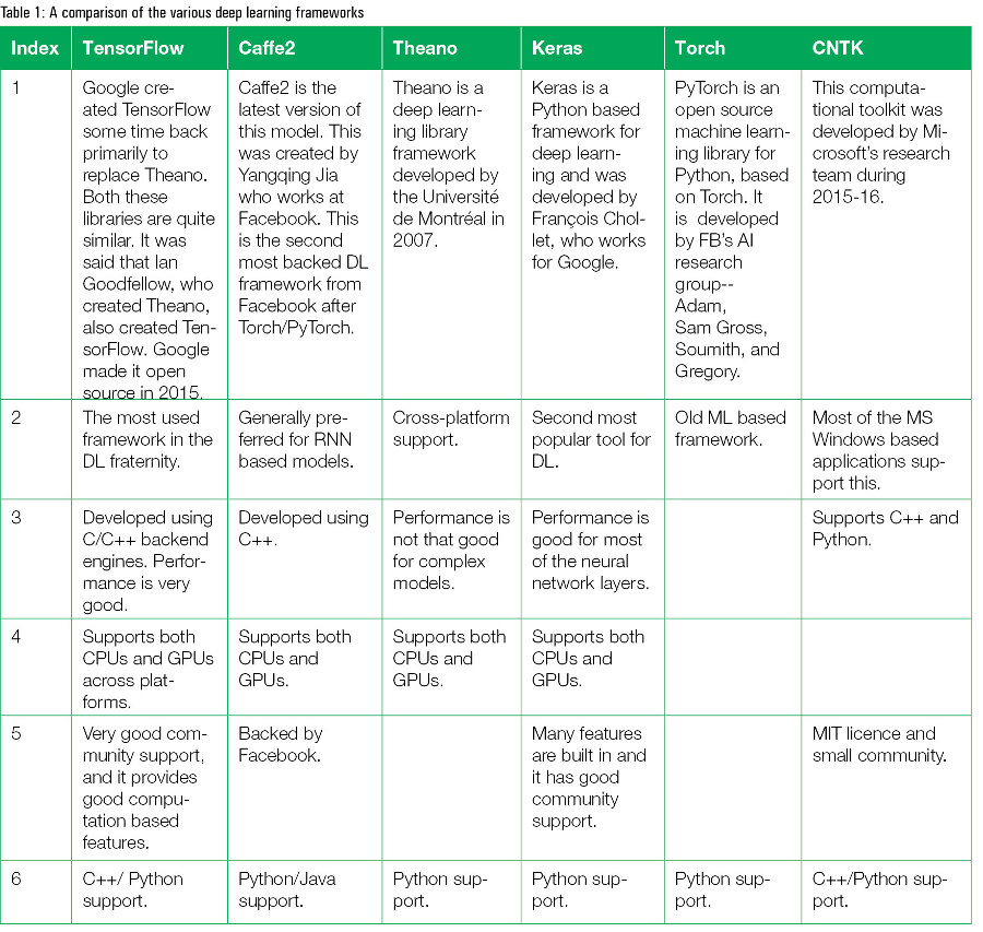
Let’s assume the reader has the requisite knowledge of deep learning models and algorithms. There are various frameworks that are used to build these deep learning (neural networks) models, with TensorFlow and Keras being the most popular. Figures 1 and 2 show the adoption levels and the support community for all these frameworks.
 TensorFlow
TensorFlow code depicts ‘computations’ and doesn’t actually perform them. To run or execute TensorFlow code, we need to create ‘tf.Session’ objects in Python.
Tensors: Tensors are mathematical constructs used especially in fields like physics and engineering. Traditionally, tensors have made less inroads into computer science. All these years computer science was more related to discrete mathematics and logical reasoning. But recent developments in machine learning have changed all that, and introduced the vector based mathematics and calculus of tensors. Here are a few basics:
1) Scalars are rank-0 tensors.
2) A Rank-1 tensor is a simple vector —all row vectors (1,2) and column vectors (2,1) are of these shapes.
3) A Rank-2 or 2D tensor is a simple 2X2 matrix. An example is: co-ordinates of a plane. A black and white image can be a 2D tensor.
4) Similarly, we have Rank-3 or 3D tensors and Rank-4 or 4D tensors, etc. A colour image of size (255,255, 3) is a 3D tensor (Note: RGB is a three-colour channel). A video of a few minutes duration is an example of a 4D tensor, assuming that we have 60 frames per second, and RGB channels the size of (255, 255, 3, 3600).
 Note: The respective version of TensorFlow can be installed on your select choice of environment like Anaconda and Jupyter notebooks, Spyder, or any select framework that supports TensorFlow. The latest supported and stable version of TensorFlow is r1.13 or r1.12. TensorFlow 2.0 Alpha is also available now.
Note: Make sure the respective Python version and matching TensorFlow version are both installed in your environment.
TensorFlow is loaded with computational as well as basic features like:
- Constants
- Variables
- Placeholders
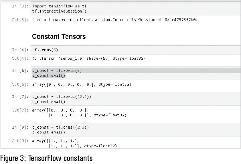
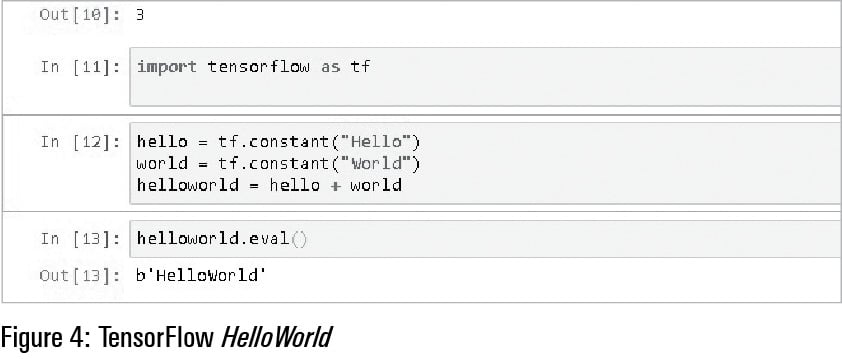
Constants: The value of constants does not change. For example, in the ‘Hello World’ code we have initialised two constants and the value is fixed.
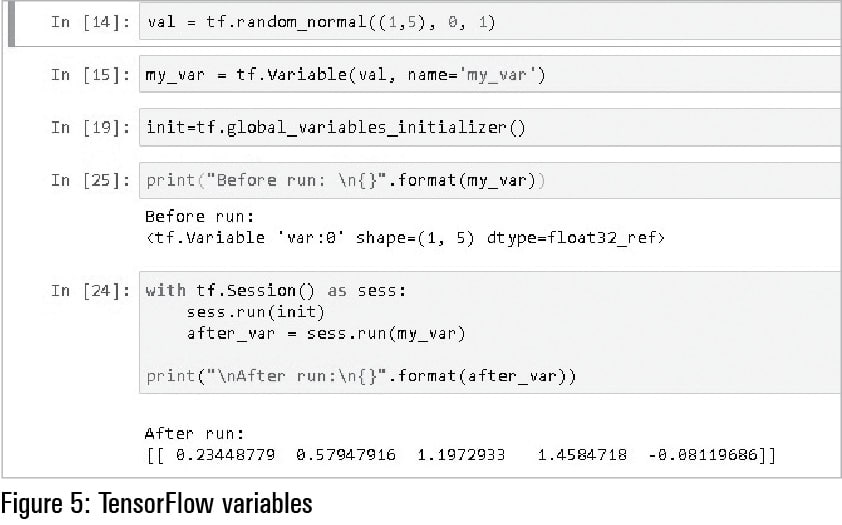
 Variables: These are objects in TensorFlow, of which the value will be ‘re-filled’ every time they are called or run in a session. These variables will maintain a fixed state in a graph. The tf.Variable() is used to declare or call variables in TensorFlow.
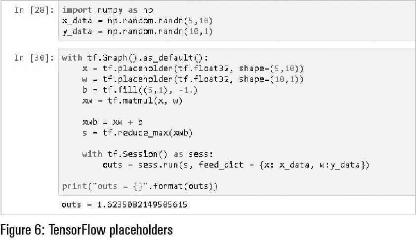
Placeholders: These are built-in structures for feeding input data. Sometimes these are thought of as empty variables that will be filled with data in the future. Placeholders have an optional ‘shape’ argument. The default option is None; otherwise, it will be assumed to be of any size.
Sessions in TensorFlow: Any tensor must reside in the computer memory in order to be useful to computer programmers. Once this interactive session is loaded, we are good to program. tf.InteractiveSession() is used to start the session and until we close or come out of this window, this session will be live.
Figures 3, 4, 5 and 6 show the usage of constant, Hello World of TensorFlow, variables and placeholders with examples in the Jupyter notebook.
 TensorFlow graphs
TensorFlow has inbuilt features that help us to build algorithms, and computing operations that assist us to interact with one another. These interactions are nothing but graphs, also called computational graphs.
TensorFlow optimises the computations with the help of the graphs’ connectivity. Each of these graphs has its own set of nodes and dependencies. Each of the types in TensorFlow — like constants, variables and placeholders — creates graphs for connectivity and computation.
Here is a coding example of linear regression using random variable generation:
import tensorflow as tf
print(tf.__version__)
import numpy as np
import matplotlib.pyplot as plt

%config InlineBackend.figure_format = ‘svg’

C:\Users\Sony\Anaconda3\lib\site-packages\h5py\__init__.py:34: FutureWarning: Conversion of the second argument of issubdtype from `float` to `np.floating` is deprecated. In future, it will be treated as `np.float64 == np.dtype(float).type`.

from ._conv import register_converters as _register_converters

1.10.0

# Below are hyper parameters like learning rate, number of epochs, number of samples
learning_rate = 0.01
epochs=100
n_samples = 30

train_x = np.linspace(0, 20, n_samples)
train_y = 3 * train_x + 4 * np.random.randn(n_samples)
## Plot before starting the training
plt.plot(train_x, train_y, ‘x’)
plt.plot(train_x, 3 * train_x)
plt.show()

# Initialize training weights in placeholder
X = tf.placeholder(tf.float32)
Y = tf.placeholder(tf.float32)

# Now initialize training biases
W = tf.Variable(np.random.randn(), name =’weights’)
B = tf.Variable(np.random.randn(), name=’bias’)
# The prediction can be based input X, Weight W and bias B
prediction = tf.add(tf.multiply(X, W), B)

# Cost function(To minimize the loss as much as possible)
# Use mean square error

cost = tf.reduce_sum((prediction - Y) ** 2) /(2 * n_samples)

optimizer = tf.train.GradientDescentOptimizer(learning_rate).minimize(cost)

#Global initializer for Tensorflow variables

init = tf.global_variables_initializer()
# tf.session for all the computation
# here the no.of epochs are run

with tf.Session() as sesh:
sesh.run(init)

for epoch in range(epochs):
for x, y in zip(train_x, train_y):
sesh.run(optimizer, feed_dict = {X: x, Y:y})

if not epoch % 20:
c = sesh.run(cost, feed_dict={X:x, Y:y})
w = sesh.run(W)
b = sesh.run(B)

print(f’epoch: {epoch:04d} cc={c:.4f} w={w:.4f} b={b:.4f}’)
weight = sesh.run(W)
bias = sesh.run(B)
plt.plot(train_x, train_y, ‘o’)
plt.plot(train_x, weight * train_x + bias)
plt.show()

epoch: 0000 cc=5.4618 w=2.3091 b=0.3990
epoch: 0020 cc=0.0384 w=3.1360 b=0.4447
epoch: 0040 cc=0.0381 w=3.1375 b=0.4217
epoch: 0060 cc=0.0378 w=3.1389 b=0.3999
epoch: 0080 cc=0.0375 w=3.1402 b=0.3792


