


For various reasons, physicists often need to plot field lines of static charges or magnetic fields. This can be done beautifully using Python. A Python GUI makes the plotting simple and easy.
In layman’s terms, the graphical user interface (GUI) is a series of labels, buttons, text boxes and many other widgets. The conventional way of taking inputs from users is through the shell of a compiler. The GUI gives programming a professional look and takes inputs from the user through a separate window.
This is an article about plotting the field lines of static charges. In books on electrostatics and magnetism, generally a plot of the field lines of a dipole is given, but rarely is anything beyond dipoles looked at. This program will help in visualising the plot of as many charges as possible within the limits of a certain coordinate axis.
We have used the IDLE 3.5.2 IDE (integrated development environment) for this program.
Concepts used
NumPy provides tools such as:
- An array object of arbitrary homogeneous items
- Fast mathematical operations over arrays
- Linear algebra, Fourier transforms, random number generation
SciPy provides a scientific computing package for Python. It imports all the functions from the NumPy namespace.
Tkinter GUI
A range of user friendly GUIs is available in Python. Some of them are Tkinter, wxPython, PythonWin, PyQt, PyGTK, Java Swing, etc. The most famous graphics module in Python is Tkinter.
Tkinter offers a wide variety of widgets for a graphical user interface, including Frame, Label, Entry, Text, Canvas, Button, Radiobutton, Checkbutton, Scale, Listbox, Scrollbar, OptionMenu, Spinbox, LabelFrame and PanedWindow.

Class
A class is the building block of object oriented programming (OOP) in Python, and is initialised by using the class keyword.
A class is a data type that has its methodology of functioning and its attributes are defined by the programmer. Whenever a class is created, it creates its own namespace, which is a set of names pertaining to that class. Whenever that class is then called by the programmer, it is termed an instantiation of that class.
A method is any attribute (function or object) that already belongs to the class and is accessed using an attribute reference. Usually, when creating an instance of a class in a program, the class has some initial values for the internal data and this is done by defining the __init__ method.
For example:
class Charge:

def __init__(self, x, y, mag):

self.x = x

self.y = y

self.mag = mag
For a field line plot, we require the descriptions of charges like position and magnitude (putting the + or – sign will take care of the type of charge), which were taken from the user with the help of a GUI built using the Tkinter module in Python.
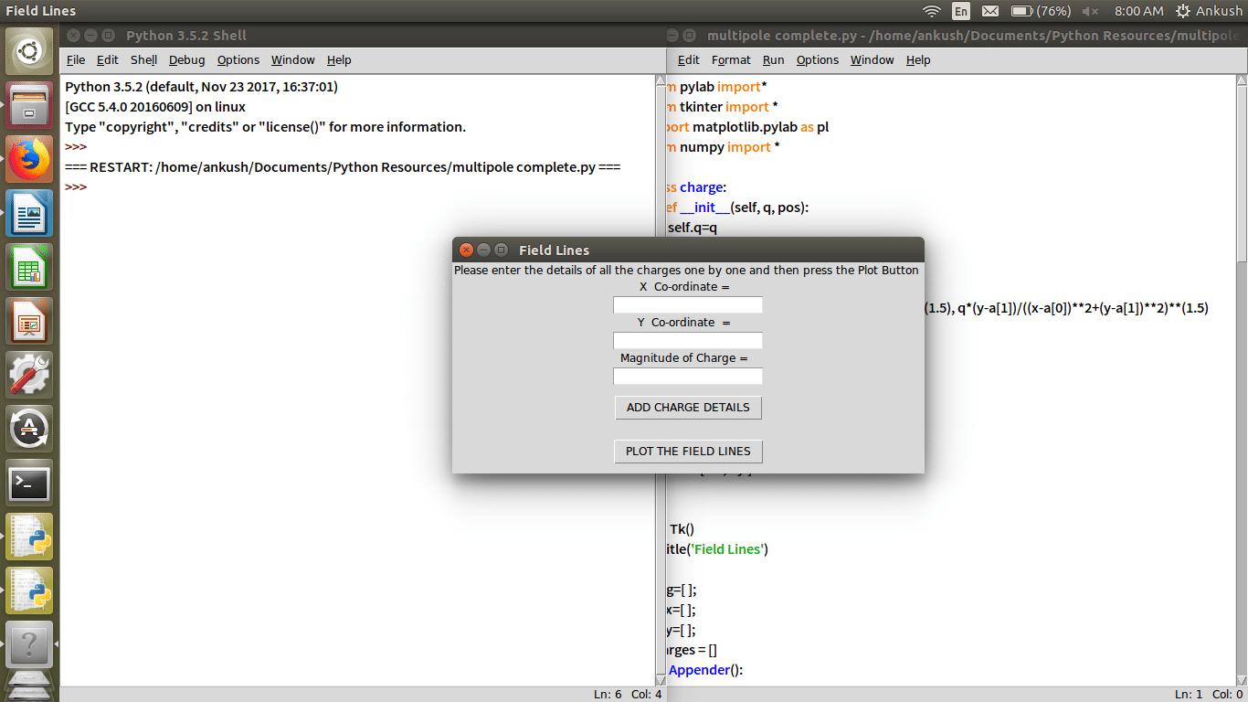
from pylab import* #* represents all submodules

from tkinter import *

import matplotlib.pylab as pl

from numpy import *

class charge:

def __init__(self, q, pos):

self.q=q

self.pos=pos

def E_point_charge(q, a, x, y):

return q*(x-a[0])/((x-a[0])**2+(y-a[1])**2)**(1.5), q*(y-a[1])/((x-a[0])**2+(y-a[1])**2)**(1.5)

# formula to calcuate electric field due to a single charge

def E_total(x, y, charges):

Ex, Ey=0, 0

for C in charges:

E=E_point_charge(C.q, C.pos, x, y)

Ex=Ex+E[0]

Ey=Ey+E[1]

return [ Ex, Ey]

w = Tk()

# creating a graphical user interface window. Figure 1.

w.title(‘Field Lines’)

#The name for a graphical user interface window Figure 1.

mag=[ ];

#List to store the magnitude of charges.

plax=[ ];

#List to store the x coordinate of charges.

play=[ ];

#List to store the y coordinate of charges.

charges = []

def Appender():

x1 = (eval(xv.get()))

x1 = float(x1)

plax.append(float(x1))

y1 = (eval(yv.get()))

y1 = float(y1)

play.append(float(y1))

mag1 = (eval(magv.get()))

mag1 = float(mag1)

mag.append(float(mag1))

c = len(plax)

pos=[];

cx=float(plax[c-1]);

pos.append(cx);

cy=float(play[c-1]);

pos.append(cy);

cm=float(mag[c-1]);

charges.append(charge (cm,pos))

space = Label(w, text = “Please enter the details of all the charges one by one and then press the Plot Button “).pack()

Xentry = Label(w, text = “X Co-ordinate = “ ).pack()

xv = StringVar()

xentry = Entry(w, text variable = xv , font=(“Sitka Text”,10)).pack()

Yentry = Label(w, text = “Y Co-ordinate = “ ).pack()

yv = StringVar()

yentry = Entry(w, textvariable = yv, font=(“Sitka Text”,10)).pack()

MAGentry = Label(w, text = “Magnitude of Charge = “ ).pack()

magv = StringVar()

magentry = Entry(w, textvariable = magv, font=(“Sitka Text”,10)).pack()

load = Button(w, text = ‘ADD CHARGE DETAILS’, command = Appender).pack(pady=10)

def Plotter():

# plot field lines

x0, x1=-10, 10

y0, y1=-10, 10

x=linspace(x0, x1, 64)

y=linspace(y0, y1, 64)

x, y=meshgrid(x, y)

Ex, Ey=E_total(x, y, charges)

streamplot(x, y, Ex, Ey, color=’k’)

# plot point charges

for C in charges:

if C.q>0:

plot(C.pos[0], C.pos[1], ‘bo’, ms=8*sqrt(C.q))

if C.q<0:

plot(C.pos[0], C.pos[1], ‘ro’, ms=8*sqrt(-C.q))

xlabel(‘$x$’) #labelling x axis

ylabel(‘$y$’) # labelling y axis

gca().set_xlim(x0, x1)

gca().set_ylim(y0, y1)

show()

ploted = Button(w, text = ‘PLOT THE FIELD LINES’, command = Plotter).pack(pady = 10)
How to use the code
Make sure that the Tkinter module is available in the IDE being used. If it is not, you can download it, based on your operating system. Once the GUI opens on running the code, the details are to be entered independently—like the position of the charge and the magnitude for each charge; and the add charge details button should be pressed. This should be done for all the charges you want, one by one, and after successively adding charges when the plot field lines button is pressed, the field lines are plotted for the set of charges.
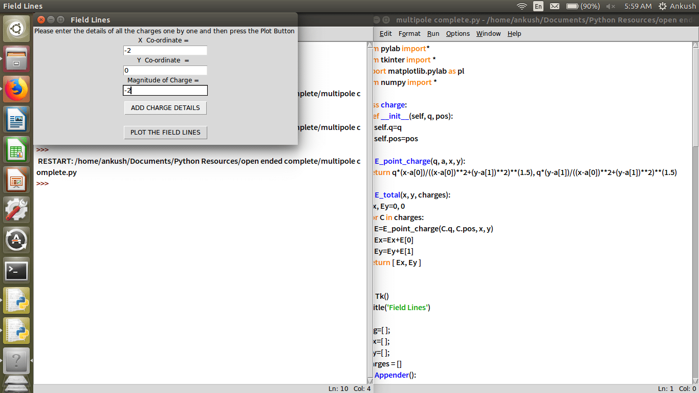
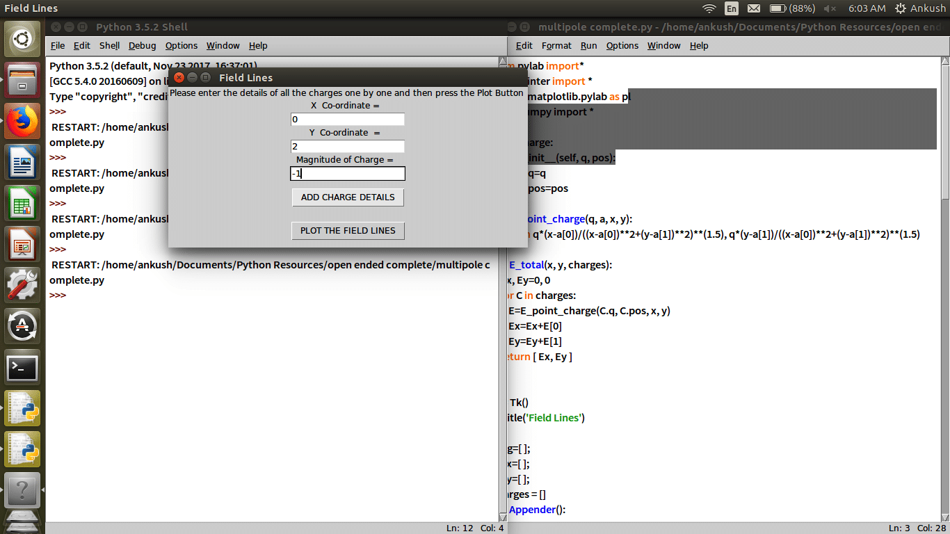
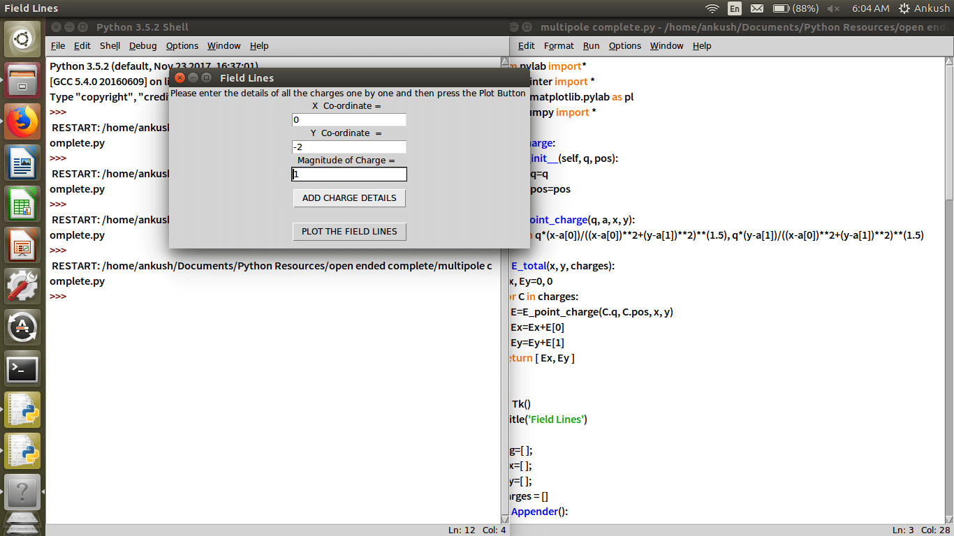
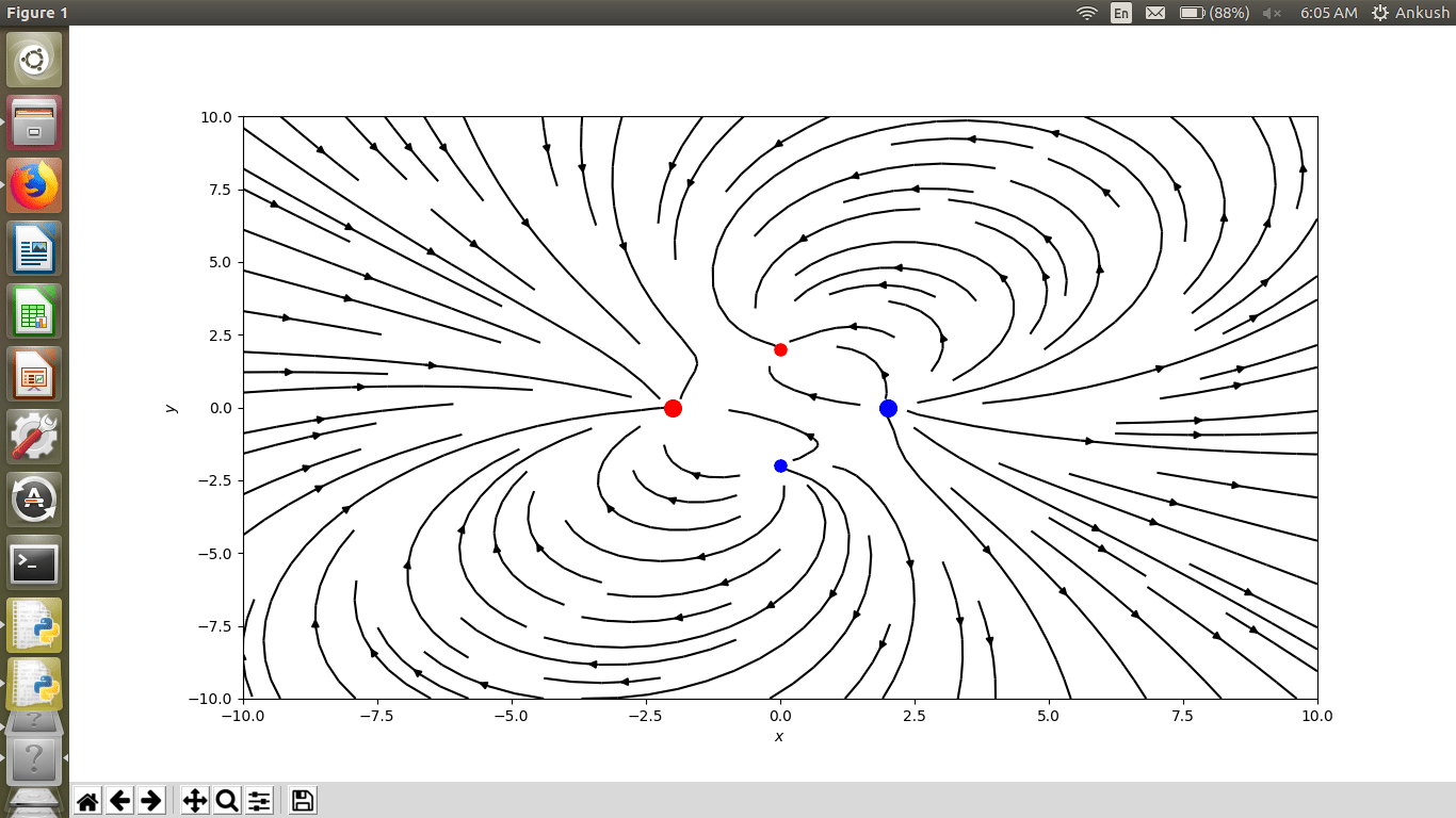
For example, for a system of four charges, the steps involved in obtaining the field lines can be seen from Figures 2 to 5. In Figure 2, the first charge has (-2, 0, -2) as its x-coordinate, y-coordinate and charge magnitude. In Figure 3, the second charge has (2, 0, 2) as its x-coordinate, y-coordinate and charge magnitude. The third and fourth charges in Figures 4 and 5 have (0, 2, -1) and (0, -2, 1), respectively, as their x-coordinate, y-coordinate and charge magnitude.
The plot of field lines obtained for this system of charges can be seen in Figure 6. For any system of static charges, field lines can be plotted in this manner.
The code shown isn’t perfect and can always be made more efficient based on one’s needs.


