Public opinion is important to enterprises, politicians, governments, film stars and most of us. Opinions can be found on various social media sites. This article demonstrates how popular sentiments can be mined from Twitter with the help of the R programming language.
Opinion mining is an area of text mining where data analytics extracts opinions, emotions and sentiments from a corpus of text. That is why it is also known as sentiment analysis. One of the most common applications of opinion mining is to track the attitudes and moods on the Web, especially to survey the status of products, services, brands or even the consumers. The main purpose is to know whether what is being surveyed is viewed positively or negatively by a given audience.
The R language supports the entire text mining paradigm with its various packages. We will discuss only opinion mining on Twitter data here, and only through packages which concern this topic.
To begin with, let’s consider the Sentiment package of Timothy Jurka. The package sentiment_0.1.tar.gz is available on https://cran.r-project.org/src/contrib/Archive/sentiment/. After downloading it, install the package with load_all(). The Sentiment package supports different tools to analyse the text corpus, and assigns weightage to each sentence on the basis of the sentiment values of different emotional keywords. Since micro bloggers use Twitter to express their thoughts in a casual way, it is a good place for sentiment analysis on different current topics. This information is gathered on the basis of different emotional keywords within the Twitter text. There are two functions that analyse the sentiment measure of a sentence.
1. The function classify_emotion() helps us to analyse some text and classify it under different types of emotions. The predefined emotions are anger, disgust, fear, joy, sadness, and surprise. Classifying text into these categories is done using one of the following two algorithms:
- The Naive Bayes classifier trained on Carlo Strapparava and Alessandro Valitutti’s emotions lexicon
- The voter procedure
2. The classify_polarity() function performs the classification on the basis of some symbolic enumeration values. The symbolic values are defined as very positive, positive, neutral, negative, and very negative. In this case also, there are two algorithms:
- The Naive Bayes algorithm trained on Janyce Wiebe’s subjectivity lexicon
- The voter algorithm.
Readers can select any one of them.

To discuss the technicality of opinion mining with R here, I have carried out an exercise using the micro-blogger site Twitter. As mentioned earlier, the reason is obvious; Twitter comments are made up of just a little text and contain informal communication. Analysis of their sentimental value is easier than of a formal text. For instance, if we consider a formal film review, we will find a well-designed analysis of the product, but the personal, casual emotions of the writer will be absent.
Preparation
The preparation for this sentiment analysis involves two stages. The first is to install and load all packages of Twitter for Twitter JSON connectivity. After this, install and load packages related to opinion mining.
Preparation for Twitter
Twitter connectivity and reading requires the following three packages. If not already installed, install them. Then, load the libraries, if the packages have been installed properly.
install.packages(“twitteR”)

install.packages(“ROAuth”)

install.packages(“modeest”)

library(twitteR)

library(“ROAuth”)

library(“httr”)

Preparation for text mining and sentiment analysis
For sentiment analysis, I have downloaded the sentiment package and loaded it as shown below. The remaining relevant packages are installed and loaded as discussed earlier.
library(devtools) #devtools contain load_all

load_all(“sentiment”) # This package require tm and NLP

install.packages(“tm”)

install.packages(“plyr”)

install.packages(“wordcloud”)

install.packages(“RColorBrewer”)

install.packages(“stringr”)

install.packages(“openNLP”)

library(tm)

library(plyr)

library(ggplot2)

library(wordcloud)

library(RColorBrewer)

library(sentiment)
Twitter connectivity
I have considered a predefined twitter application account to access the twitter space. Interested readers should create their own account to view this opinion mining experiment. You may refer earlier article from OSFY Jan 2018 issue.
download.file(url=”http://curl.haxx.se/ca/cacert.pem”,destfile=”cacert.pem”)

cred<- OAuthFactory$new(consumerKey=’HTgXiD3kqncGM93bxlBczTfhR’,

consumerSecret=’djgP2zhAWKbGAgiEd4R6DXujipXRq1aTSdoD9yaHSA8q97G8Oe’,

requestURL=’https://api.twitter.com/oauth/request_token’,

accessURL=’https://api.twitter.com/oauth/access_token’,

authURL=’https://api.twitter.com/oauth/authorize’)

# enter PIN FROM https://api.twitter.com/oauth/authorize

cred$handshake(cainfo=”cacert.pem”)
This handshaking protocol requires PIN number verification, so enter your PIN as shown in the Twitter logged-in screen. Saving Twitter authentication data is a helpful step for future access to your Twitter account.
save(cred, file=”twitter authentication.Rdata”)

consumerKey=’HTgXiD3kqncGM93bxlBczTfhR’

consumerSecret=’djgP2zhAWKbGAgiEd4R6DXujipXRq1aTSdoD9yaHSA8q97G8Oe’

AccessToken<- ‘1371497582-xD5GxHn kpg8z6k0XqpnJZ3XvIyc1vVJGUsDXNWZ’

AccessTokenSecret<- Qm9tV2XvlOcwbrL2z4Qkt A3azydtgIYPqflZglJ3D4WQ3’

setup_twitter_oauth(consumerKey, consumerSecret,AccessToken,AccessTokenSecret)
Analysis of text: Create a corpus
To perform a proper sentiment analysis, I have selected the popular ‘Women’s reservation’ topic, and analysed the Twitter corpus to study the sentiments of all the participants with a Twitter account. To have a locality search within India, I have set the geocode at Latitude: 21.146633 and Longitude: 79.088860, within a radius of 1000 miles (Figure 1).
In total, 1500 tweets with the given keyword have been selected using the function searchTwitter().
# read tweets word

read_tweets = searchTwitter(“womens+reservation”, n=1500, lang=”en”,geocode=’21.14,79.08,1000mi’)
The + sign within the search string indicates a search for both the strings.
# extract the text from tweets

tweeter_txt = sapply(read_tweets, function(x) x$getText())
Since Twitter data often contains special characters along with different graphical icons, it is required to filter out all non-alphabetic content from the tweets. This filtering has been done by removing retweets, @, punctuations, numbers, HTML links, extra white spaces and all the crazy characters. To make all the text uniform, globally, everything has been converted to lower case letters. Finally, all the NAs have been removed and the header tag names made empty with NULLs.
# remove at people

twitter_txt = gsub(“@\\w+”, “”, twitter_txt)

#”crazy” characters, just convert them to ASCII

twitter_txt = iconv(twitter_txt, to = “ASCII//TRANSLIT”)

#Create a corpus from the twitter data

docsCorpus <- Corpus(VectorSource(twitter_txt))

#remove all Punctuation

docsNoPunc<- tm_map(docsCorpus, removePunctuation)

#Remove all numbers

docsNoNum<- tm_map(docsNoPunc, removeNumbers)

# Convert all to lower case

docsLower <- tm_map(docsNoNum, tolower)

# remove stop words

docsNoWords<- tm_map(docsLower, removeWords, stopwords(“english”))

#remove space

docsNoSpace<- tm_map(docsNoWords, stripWhitespace)

# Convert corpus to text

docsList = lapply(docsNoSpace,as.character)

twitter_txt = as.character(docsList)

# Replace all attributes to NULL

names(twitter_txt) = NULL
The next task is to classify the Twitter corpus into different classes. For this, I have used the Bayesian algorithm with prior equal to 1. In this case, the emotion classifier will try to evaluate each sentence with respect to its six sentiment measures, and will finally assign a classification measure to each sentence. All the unclassified sentences are categorised as NA and are finally marked as ‘unknown’.
# classify emotion

class_emo = classify emotion(twitter_txt, algorithm=”bayes”, prior=1.0)

# get emotion best fit

>head(class_emo,1)

ANGER DISGUST FEAR

[1,] “1.46871776464786” “3.09234031207392” “2.06783599555953”

JOY SADNESS SURPRISE BEST_FIT

[1,] “1.02547755260094” “1.7277074477352” “2.78695866252273” NA

emotion = class_emo[,7]

# substitute NA’s by “unknown”

emotion[is.na(emotion)] = “unknown”
Classification of sentences requires the polarity measure of each sentence on the basis of its sentiment values. There are three sentiment measures — neutral, positive and negative. The polarity measure function classify_pol() assigns one of these three sentiment measures to each sentence. This function uses the Bayesian algorithm to calculate the final sentiment polarities of each sentence of the corpus.
# classify polarity

class_pol = classify_polarity(twitter_txt, algorithm=”bayes”)

>head(class_pol,1)

POS NEG POS/NEG BEST_FIT

[1,] “24.2844130953411” “18.5054868578024” “1.3122817725329” “neutral”

# get polarity best fit

polarity = class_pol[,4]

For final statistical analysis of these sentiment values, convert the corpus into the most convenient data structure of R, i.e., a data frame. This contains both the emotion and polarity values of the Twitter corpus.
sent_df = data.frame(text= twitter_txt, emotion=emotion,

polarity=polarity, stringsAsFactors=FALSE)

# sort data frame

sent_df = within(sent_df,

emotion<- factor(emotion, levels=names(sort(table(emotion), decreasing=TRUE))))
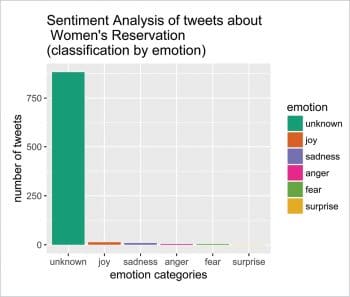
A histogram plot of the distribution of emotions is helpful to get a perceptual idea of sentiment distribution within the Twitter corpus. Figure 2 gives a demonstration of this distribution plot, using the ggplot() function.
# plot distribution of emotions

ggplot(sent_df, aes(x=emotion)) +

geom_bar(aes(y=..count.., fill=emotion)) +

scale_fill_brewer(palette=”Dark2”) +

xlab(“emotion categories”) + ylab(“number of tweets”) +

ggtitle(“Sentiment Analysis of tweets about\n Women’s Reservation \n(classification by emotion)”) + theme (text = element_text ( size = 12 , family=”Impact”))
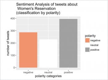
Similar to sentiment distribution, we may have a polarity distribution of the corpus from the histogram plotting of the polarity values of the data frame sent_df (Figure 3).
ggplot(sent_df, aes(x=polarity)) +

geom_bar(aes(y=..count.., fill=polarity)) +

scale_fill_brewer(palette=”RdGy”) +

xlab(“polarity categories”) + ylab(“number of tweets”) +

ggtitle(“Sentiment Analysis of tweets about \n Women’s Reservation \n(classification by polarity)”) + theme ( text = element_text ( size = 12 , family = “Impact” ) )
It can be seen that both these frequency distribution histograms are quite useful graphical depictions of the sentiments of 1500 tweets spread over the Indian subcontinent. As expected, the largest number can be categorised as unclassified, but the remaining values are quite helpful to get a clear idea of an individual’s feelings about the subject of debate. The analysis is based on some predefined emotion categories and the vocabulary of the test database is also limited; so there are ample opportunities for improvement.


