Deep (machine) learning: Everything you need to know about it

 

For years, humans have tried to get computers to replicate the thinking processes of the human brain. To a limited extent, this has been possible by using deep learning and deep neural networks. This article provides insights into deep or machine learning.

When surfing the Net or while on social media, you must have wondered how you automatically get pop-ups of things that interest you. Did you know that there are lots of things happening behind the scenes? In fact, lots of computations and algorithms are running in the background to automatically find and display things that interest you, based on your search history… And this is where deep learning begins.

Deep learning is one of the hottest topics nowadays. If you do a Google search, you will come across a lot that’s happening in this field and it is getting better every day, as one can gauge when reading up on, ‘Artificial intelligence: Google’s AlphaGo beats Go master Lee Se-dol’.

In this article, we will look at how we can practically implement a three-layer network for deep learning and the basics to understand the network.

Definition

It all started with machine learning – a process by which we humans wanted to train machines to learn as we do. Deep learning is one of the ways of moving machine learning closer to its original goal—artificial intelligence.

As we are dealing with computers here, inputs to these are data such as images, sound and text. Problem statements include image recognition, speech recognition, and so on. We will focus on the image recognition problem here.

History

When humans invented computers, scientists started working on machine learning by defining the properties of objects. For instance, the image of a cup was defined as cylindrical and semi-circular objects placed close to each other. But in this universe, there are so many objects and many of them have similar properties. So expertise was needed in each field to define the properties of the objects. This seemed to be a logically incorrect method as its complexity would undoubtedly increase with an increase in the number of objects.

This triggered new ways of machine learning whereby machines became capable of learning by themselves, which in turn led to deep learning.

Architecture

This is a new area of research and there have been many architectures proposed till now. These are:

1. Deep neural networks
2. Deep belief networks
3. Convolutional neural networks
4. Convolutional deep belief networks
5. Large memory storage and retrieval (LAMSTAR) neural networks
6. Deep stacking networks

Deep neural networks (DNNs)

Let us now look at how deep neural networks work.

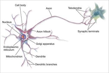
The word ‘neural’ in DNN is related to biology. Actually, the soul of these networks is how the biological neural system works. So, let’s take a brief look at how two biological neurons communicate.

There are three main parts in a biological neuron as shown in Figure 1.

1. Dendrite: This acts as input to the neuron from another neuron.
2. Axon: This passes information from one neuron to another.
3. Synaptic connection: This acts as a connection between two neurons. If the strength of the received signal is higher than some threshold, it activates another neuron.

Neuron types

Let us try to express human decisions and biological neural networks mathematically so that computers can comprehend them.

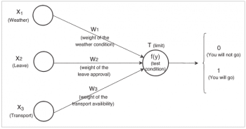
Let’s suppose that you want to go from city A to city B. Prior to making the journey, there are three factors that will influence your travel decision. These are:

1. If the weather (x1) is good (represented by 1) or bad (represented by 0) has a weight of (w1)
2. If your leave (x2) is approved (represented by 1), or not (represented by 0) has a weight of (w2)
3. If transport (x3) is available (represented by 1) or not (represented by 0) has a weight of (w3)

And you will decide as follows: Irrespective of whether your leave is approved or not and transport is available or not, you will go if the weather is good. This problem statement can be drawn as shown in Figure 2.

According to the figure, if the sum of the product of the inputs (xi) and their respective weights (wi) is greater than some threshold (T), then you will go (1), else you will not (0).

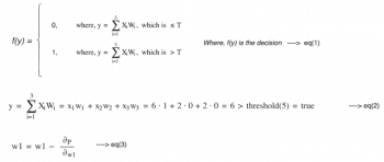As your input and output is fixed, you have to choose weights and thresholds to satisfy the equation.

For example, let us choose w1=6, w2=2, w3=2 and T=5.

You will be able to make a correct decision if we choose the above values for equation (1), i.e., if your leave is not approved (0) and transport is not available (0) but the weather is good (1), then you should be going.

Similarly, you can check other conditions as well.

It will be easy to manually calculate these weights and thresholds for small decision-making problems but as complexity increases, we need to find other ways – and this is where mathematics and algorithms come in.

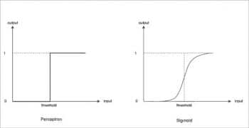
f(y), the function represented in Figure 3, produces output in terms of 0 and 1. This says that for a small change in input, the change in output is high — represented by a step function. This can cause problems in many cases. Hence, we need to define a function f(y) such that for small changes in input, changes in the output are small — represented by the Sigmoid function.

Depending upon these conditions, there are two neuron types defined, as shown in Figure 3.

Defining DNN

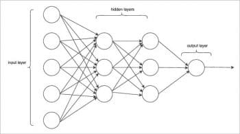
In Figure 2, Xi represents the input neuron while f(y) represents the output neuron, while layers are called the input and output layer, respectively.

In DNN, there are multiple hidden layers of units between the input and output layers, as shown in Figure 4.

Let us see how the theory discussed so far is used practically, in the following text.

Training a network

There are two stages involved in a DNN:

1. Training the network
2. Testing the network for how well it has been trained

Before we move on, let’s get familiar with the mathematical terms and definitions that we will use, going forward.

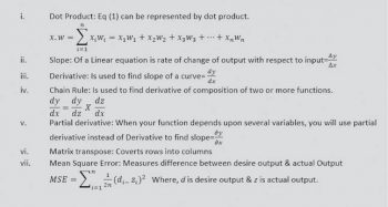
To begin with, you can refer to Box 1 for all the relevant formulae.

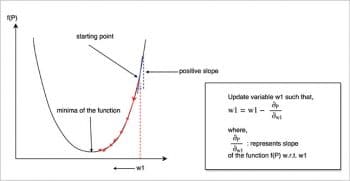
Next, the gradient descent is used to find the local minima of a function (Figure 5).

The gradient descent works as follows:

• The given performance function f(p) is dependent on w1.
• We have to calculate the minima of the function (i.e., the value for which the function is minimum).
• We randomly initialise the value of w1 to get the starting point.
• Then we calculate the slope of the function with respect to w1 and update the weight as follows:
• As per Figure 5, the slope is positive, w1 is decreasing, and we are going in the correct (i.e., downward) direction.

Back propagating errors occur from the output to the input layer.

Now, let’s look at how to implement a three-layer DNN.

Understanding problem statements

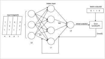
In Figure 6, we have four images in binary format given as inputs to the network. Each image is 3 bits long. With respect to each binary input, we have the input neuron defined. So there are three input neurons in the input layer. There are four neurons in the hidden layer. And one output neuron.

With respect to each image, there is a predefined desired output (d).

Assume that Images 1 and 4 are of digit 0 with the desired output-binary 0; and Images 2 and 3 are of digit 1 with the desired output-binary 1.

There are 12 weights in Layer L1 and four in Layer L2 for connection between the two layers.

As our input and output is fixed, we need to find weights in Layer L1- w1 and weights in Layer L2- w2 such that our actual output (z) is equal to the desired output (d).

Figure 6 can be drawn as a block diagram as shown in Figure 7 to derive the required equations.

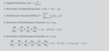
Box 2 gives different equations for DNNs.

Steps for implementing a three-layer DNN

1. Initialise the weights w1 randomly. Dot product of input-x and weights w1 produces P1, which acts as input to the Sigmoid function1 in layer L1.
2. The output of the Sigmoid function is y, which acts as input to the output layer.
3. Again, randomly initialise weights w2. The dot product of y and weights w2 produces P2, which acts as input to the Sigmoid function2 in layer L2.
4. The output of Sigmoid function2 is z, which is our actual output. Give this output to the performance function P along with the desired output to produce an error.
5. Minimise this error by backpropagating it and using the gradient descent algorithm, i.e., change weights w1 and w2 to find the minima of the performance function.
6. When the error is minimum, the actual output will be close to the desire output.

The Python code given below shows the practical implementations:

import numpy as np

import matplotlib.pyplot as plt

def nonlin(x,deriv=False):

if(deriv==True):

return x*(1-x) #derivative of the Sigmoid function

return 1/(1+np.exp(-x)) #Sigmoid function

def show_error(l):

e=[];e1=[];e2=[];e3=[];e4=[]

count1=0;count2=1;count3=2;count4=3

for i in l:

for j in i:

for k in j:

e.append(k)

for i in range(10000):

e1.append(e[count1]);e2.append(e[count2]);e3.append(e[count3]);e4.append(e[count4])

count1+=4;count2+=4;count3+=4;count4+=4

plt.plot(e1,label='input1');plt.plot(e2,label='input2');plt.plot(e3,label='input3');plt.plot(e4,label='input4')

plt.xlabel('Iteration',fontsize=17);plt.ylabel('Error',fontsize=17)

plt.legend();plt.grid(True)

plt.show()

x = np.array([[0,0,1], #input dataset

[0,1,1],

[1,0,1],

[1,1,1]])

d = np.array([[0], #desire output dataset

[1],

[1],

[0]])

np.random.seed(1)

w1 = 2*np.random.random((3,4)) - 1 #Randomally initializing weights in Layer1

w2 = 2*np.random.random((4,1)) - 1 #Randomally initializing weights in Layer2

l=[] #list

for j in xrange(10000): #Find slop/Derivative for n number of steps

l0 = x

y = nonlin(np.dot(l0,w1)) #dot product of inputs and weights are given to Sigmoid function which produces output y

z = nonlin(np.dot(y,w2)) #dot product of inputs and weights are given to Sigmoid function which produces output z

p = z - d #Error

l2_delta = p*nonlin(z,deriv=True)

l1_error = l2_delta.dot(w2.T)

l1_delta = l1_error * nonlin(y,deriv=True)

w2 -= y.T.dot(l2_delta) #new_weight(w2)=old_weight(w2)-change in weight(i.e.derivative w.r.t w2)

w1 -= l0.T.dot(l1_delta) #new_weight(w1)=old_weight(w1)-change in weight(i.e.derivative w.r.t w1)

arry_to_list=p.tolist()

l.append(arry_to_list)

show_error(l)

The basic code is taken from https://iamtrask.github.io/2015/07/27/python-network-part2/ and updated for the practical understanding of the learning rate and graph output.

Output

After adding debug prints, we get the output as shown in the box below, for the above program. You can see that after training is complete, the error is almost zero and the actual output is close to the desired output.

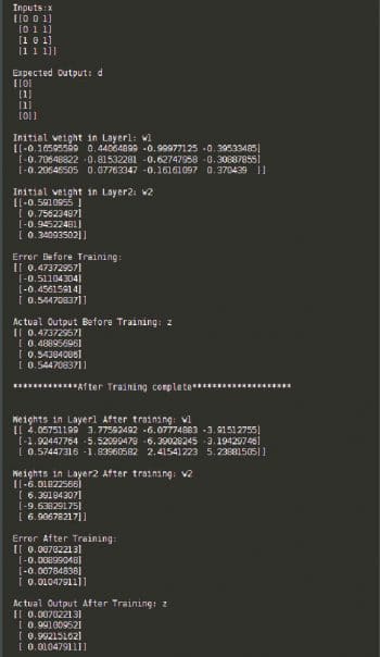If you use the weights that we get after training and the new input (other than those that we used in training), you will get the actual output in terms of trained inputs only.

If you closely look at the code, the main things are happening at Lines 63 and 65. These two lines are just using the derivation equations derived in Box 2.

Learning rate

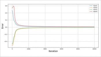
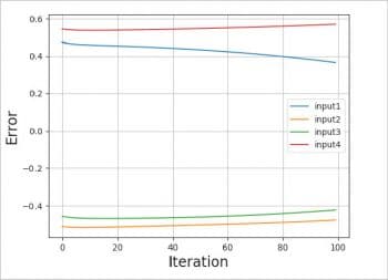
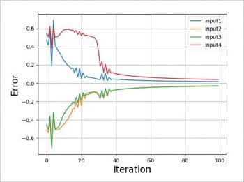
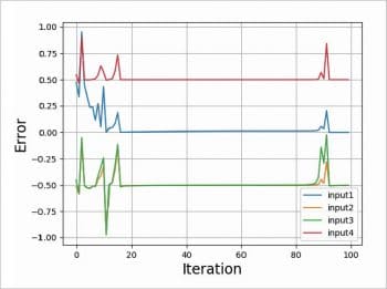
Please refer to Figures 8, 9, 10 and 11. The graphs given in these figures are plotted for different test scenarios by slightly modifying the code.

Case 1 (Figure 8)

• Keep updating weights by calculating the slope for 10,000 iterations (same as code above).
• We actually don’t need these many iterations to reach an error close to zero.

Case 2 (Figure 9)

• If the number of iterations is too low, in our case, 100, we will not get an error close to zero. And our actual output will not be close to the desired output. It will be unpredictable.

Case 3 (Figure 10)

• There is a way with which we can reduce the error close to zero for a small number of iterations. The only update you will need is to multiply the slope by some constant.
• Here, I used the constant 20, which is called the learning rate.

Case 4 (Figure 11)

• You cannot make the learning rate too small or too big.
• If the learning rate is too big (I used 50), there is the possibility of the system becoming unstable, as shown in Figure 11.
• If the learning rate is too small, the learning time will increase

I would like to conclude the article by discussing the computing power needed in building large DNNs, and where the world is headed in this area. The average human brain has 100 billion neurons while one of the artificial DNNs which won the Imagenet competition had 650,000 neurons.

With the increase in the number of neurons, the complexity increases and hence there is a need for more computation. The examples given above train in a few milliseconds. DNNs with millions of neurons and high training datasets (inputs) take months and years to train a network on a CPU. We can reduce this training time drastically by using GPUs.

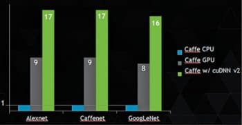
Some comparative data is given in Figure 12. Here, cuDNN v2 performance is compared with CAFFE using several well-known networks. The CPU is 16-core Intel Haswell E5-2698 2.3GHz with 3.6GHz Turbo. The GPU is NVIDIA GeForce GTX TITAN X.

(The NVIDIA CUDA Deep Neural Network library (cuDNN) is a GPU-accelerated library of primitives for deep neural networks to help increase their performance. The latest cuDNN v4 library yields more performance.)

All major tech companies such as Google, Facebook, IBM, Apple, etc, (the list is too big to cover here) are moving to deep learning nowadays, and using it for applications that range from speech recognition to self-driving cars.