Scilab has solutions for standard and large scale optimisation problems in engineering. It provides algorithms to solve constrained, unconstrained, continuous and discrete problems.
Optimisation occurs in nature all around us. Water droplets optimise themselves into a sphere, which is the least possible area for any given volume. Migrating flock of birds optimises its use of energy by flying in a V-shaped formation, which reduces air resistance. We continuously learn from nature to artificially engineer things like the honeycomb structure or the flight formation of fighter jets.
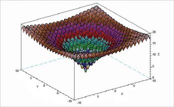
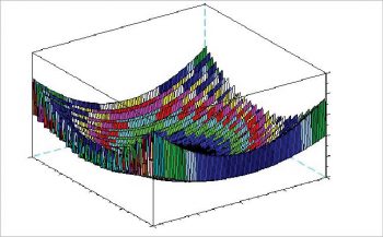
To optimise engineering objectives, we use toy functions that are noisy, non-linear and two-dimensional as benchmarks. Scilab is one of the open source platforms in which three-dimensional (3D) plots are possible. Numerical studies followed by visual interpretation help us to understand the efficiency of proposed algorithms. Real world assumptions of engineering problems are bound to truncate broad assumptions into narrow band, making it difficult to solve them using conventional methods. These problems are solved using algorithms benchmarked with toy functions.
Some toy functions from Scilab
In a broad sense, to maximise or minimise an objective function while satisfying some constraints is said to be optimisation. Some of the main toy functions used are:
1. Ackley’s function
2. Levi function
3. Holder-table function
4. Buckin function
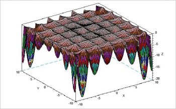
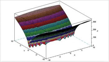
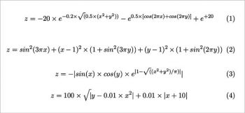
The 3D plots for these functions are shown in Figures 1, 2, 3 and 4, respectively, and the equations of each function are shown in Figure 5.
Optimisation
Here, we are concerned about minimising the constrained optimisation problem. Two dimensional functions have a pair of values as the solution. Hence, these two values determine the optimal value for the objective function/toy function. We use Firefly algorithm as optimisation algorithm for all the non-linear toy functions. Do check my article in the January 2017 edition of OSFY for Firefly algorithm and Scilab.
Interpretation
Using 50 flies scattered over Ackley’s function, approximate values of (0, 0) and the objective value of 0 is obtained as the final solution after 50 iterations. Figure 6 shows the initial stage of the 50 flies and Figure 7 shows the final stage of convergence. A dark dot at the bottom of the function is the collection of flies reaching the final minimum value of the problem; or the flies having good food, as we observe in nature. Similarly, optimal values of 0, -19.2085 and 0, respectively, are obtained for other toy functions.
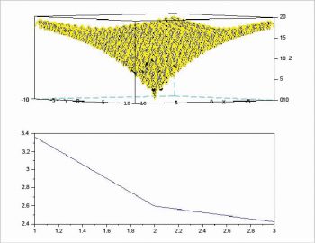
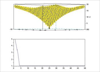
Scilab software is freely available for numerical optimisation and other computation. From Scilab, non-linear toy functions are optimised using the Firefly algorithm. The convergence of the algorithm is faster as shown in Figures 6 and 7. The trajectory for convergence using contour plots and other performances can be obtained with a few tweaks within the algorithm. For now, we have discussed the general idea of implementing toy function optimisation in Scilab.


