How to use text mining with R

The vast quantity of data, textual or otherwise, that is generated every day has no value unless processed. Text mining, which involves algorithms of data mining, machine learning, statistics and natural language processing, attempts to extract some high quality, useful information from the text.

Text mining, in general, means finding some useful, high quality information from reams of text. More specifically, text mining is machine-supported analysis of text, which uses the algorithms of data mining, machine learning and statistics, along with natural language processing, to extract useful information. It covers a wide range of applications in areas such as social media monitoring, recommender systems, sentiment analysis, spam email classification, opinion mining, etc.

Whatever be the application, there are a few basic steps that are to be carried out in any text mining task. These steps include preprocessing of text, calculating the frequency of words appearing in the documents to discover the correlation between these words, and so on. R is an open source language and environment for statistical computing and graphics. It includes packages like tm, SnowballC, ggplot2 and wordcloud, which are used to carry out the earlier-mentioned steps in text processing.

Getting started
The first prerequisite is that R and R Studio need to be installed on your machine. R Studio is an integrated development environment (IDE) for R. The free open source versions of R Studio and R can be downloaded from their respective websites.
Once you have both R and R Studio on your machine, start R Studio and install the packages tm, SnowballC, ggplot2 and wordcloud, which are usually not installed by default. These packages can be installed by going to Tools -> install packages in R Studio.

Loading data
First, let us start by loading the data, which can be any text (or collection of texts, commonly referred to as a corpus) from which we want to extract useful information. To illustrate the process in this tutorial, we have used five text documents related to our favourite superhero, Batman!
For this step, first load the library tm and then use the function Corpus() to create a collection of documents. This loads our text documents residing in a particular folder into a corpus object.

library(tm)
docs <- Corpus(DirSource(“path to your folder”))
docs
<<VCorpus>>
Metadata: corpus specific: 0, document level (indexed): 0
Content: documents: 5

The above method is to be used when you want to perform text processing on data present on your local machine in a folder, but if you want to load a dataset from an online repository, R allows you to directly load the dataset into your project as mentioned below.
To understand how to load data in R directly from the Internet, we use the famous Iris dataset (stored in CSV format) available from the UCI Machine Learning Repository (http://archive.ics.uci.edu/ml/), which provides free access to several datasets that can be used to test many machine learning algorithms.
Download and load the library RCurl which allows fetching of URIs, HTTP requests, get and post forms, and then process the results returned from the Web server, as follows:

library(RCurl)
url <-’https://archive.ics.uci.edu/ml/machine-learning-databases/iris/iris.data’
docs <- getURL(url, ssl.verifypeer=FALSE)
connection <- textConnection(docs)
dataset <- read.csv(connection, header=FALSE)
head(dataset)
V1 V2 V3 V4 V5
1 5.1 3.5 1.4 0.2 Iris-setosa
2 4.9 3.0 1.4 0.2 Iris-setosa
3 4.7 3.2 1.3 0.2 Iris-setosa
4 4.6 3.1 1.5 0.2 Iris-setosa
5 5.0 3.6 1.4 0.2 Iris-setosa
6 5.4 3.9 1.7 0.4 Iris-setosa

Preprocessing
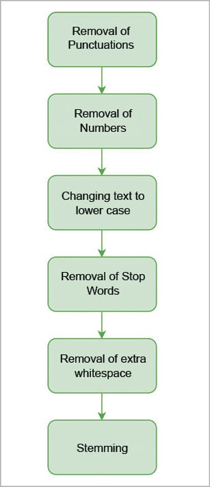
Preprocessing the text means removing punctuations, numbers, common words, etc. This step is performed to clean the data to increase the efficiency and robustness of our results by removing words that don’t necessarily contribute to our analysis.
Removal of punctuation: To remove all punctuation, use the following command:

docs <- tm_map(docs, removePunctuation)

Removal of numbers: The following command will remove the numbers in the text:

docs <- tm_map(docs, removeNumbers)

Changing the text to lower case: The command shown below will change the text being mined into lower case:

docs <- tm_map(docs, tolower)

Removal of stop words: Common words like ‘but’, ‘and’, etc, are called stop words. The following command will remove them:

docs <- tm_map(docs, removeWords, stopwords(“english”))

Removal of extra whitespaces: The following command will remove the extra whitespaces:

docs <- tm_map(docs, stripWhitespace)

Stemming: Stemming is the procedure of converting words to their base or root form. For example, playing, played, plays, etc, will be converted to play.
To perform stemming, use the command shown below:

library(SnowballC)
docs <- tm_map(docs, stemDocument)

Document term matrix
A document term matrix (DTM) depicts the frequency of a word in its respective document. In this matrix, the rows are represented by documents and the columns are represented by words. How often a word occurs in a document, is what determines the value ascribed to it—if it appears only once, its value is 1; if it appears twice, its value is 2; and if it does not appear at all, then the value is 0.
To create a DTM for our corpus, type:

dtm<- DocumentTermMatrix(docs)
dtm
<<DocumentTermMatrix (documents: 5, terms: 2566)>>
Non-/sparse entries: 3449/9381
Sparsity : 73%
Maximal term length: 23
Weighting : term frequency (tf)

The summary of our DTM states that there are five documents and 2566 unique words. Hence, let’s give a matrix with the dimensions of 5×2566, in which 73 per cent of the rows have value 0.
To get the total frequency of words in the whole corpus, we can sum the values in a row, as follows:

freq <- colSums(as.matrix(dtm))

For that, we have to first transform the DTM into a matrix, and then sum up the rows to give a single value for each column.
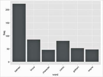
Next, we sort this in descending order to get to know the terms with the highest frequency, as follows:

ord <- order(freq,decreasing=TRUE)
freqn[head(ord)]
batman bruce comic gotham wayne character 
222 85 80 52 47 46

Finding associations
After the previous step, we get a rough idea that the terms ‘batman’, ‘bruce’, ‘comic’, ‘wayne’ and ‘character’ are central to our corpus. Thus, if we want to find terms that highly correlate with them we can use the findAssocs() function, which takes as its parameter the DTM, the word and the correlation limit (which ranges from 0 to 1). A correlation of 1 means ‘always together’, while a correlation of 0.5 means ‘together for 50 per cent of the time’.

findAssocs(dtm, “bruce”, corlimit=0.90)
$bruce
able pain times order will time 
0.99 0.98 0.98 0.97 0.96 0.95 
access day defeat earth eyes idea 
0.94 0.94 0.94 0.94 0.94 0.94 
individual minds nightwing sometimes unlike character 
0.94 0.94 0.94 0.94 0.94 0.93 
associated life part personality alfred man 
0.92 0.92 0.92 0.92 0.91 0.91 
parents 
0.91

Plotting the term frequencies
To graphically represent our term frequencies as a plot, the ggplot2 library is used as follows:

library(ggplot2) 
wf <- data.frame(word=names(freq), freq=freq)
p <- ggplot(subset(wf, freq>30), aes(word, freq))
p <- p + geom_bar(stat=”identity”) 
p <- p + theme(axis.text.x=element_text(angle=45, hjust=1)) 
p

Word Cloud
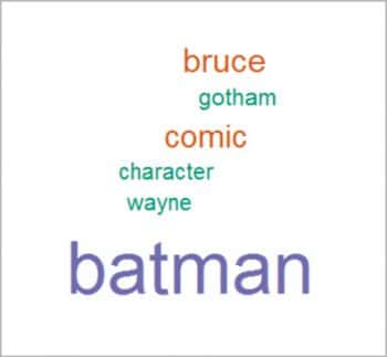
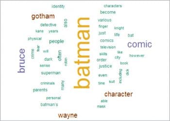
Word Cloud is another way of representing the frequency of terms in a document. Here, the size of a word indicates its frequency in the document corpus.
Load the wordcloud package, as follows:

library(wordcloud)

For Word Cloud comprising terms with a frequency greater than 30, use the following command:

wordcloud(names(freq), freq, min.freq=30,colors=brewer.pal(3,”Dark2”))

For a Word Cloud for the 50 words that occur most often, use the command given below:

wordcloud(names(freq), freq, max.words=50,colors=brewer.pal(6,”Dark2”))

Text processing is about extracting useful information from text, which includes basic steps of pre-processing data, stemming the data, representing the corpus using the document term matrix and obtaining the associations between terms. R provides several libraries and functions to efficiently carry out these tasks.