Scilab is free and open source software for numerical computation. It provides engineers and scientists with a powerful environment to do their computation.
Engineers and scientists all over the world use computers for their calculations, yet many of us remain unaware of the software or tools used by a majority of them. Since the invention of transistor in 1947, computing power has increased tremendously, more or less according to the predictions made in Moore’s Law. The law states that the number of transistors in a given area will be doubled approximately every two years. In 2015, the transistor count was 5.5 billion in an Intel processor. That is around 5.5 per cent of the 100 billion neurons in the human brain. So, artificial intelligence (AI) is getting closer to human intelligence.
MATLAB is a high level numerical computational platform with IEEE floating point precision of approximately 16 decimal digits. However, space exploration demands a greater level of decimal precision— approximately 25 digits is the count for ISRO. So do NASA and ISRO use MATLAB? Yes, they do, for most of their computation. But they also use Scilab, an open source, high level numerical computational platform.
Scilab can be downloaded from www.scilab.org. Taking up about 150MB, it can be installed on your Linux, Windows or Mac OS. Learning Scilab is easy with http://www.scilab.in and with the initiatives taken by Prof. Kannan M. Moudgalya at the Indian Institute of Technology, Bombay. The professor’s textbook companion project at www.scilab.in/Completed_Books contains almost all the engineering numerical problems solved with Scilab. These can be accessed freely, but sadly, most engineering students are unaware of this.
MATLAB
Cleve Moler, the chairman of the computer science department of the University of New Mexico, started developing MATLAB in the late 1970s. The latest release of this proprietary programming language has a memory size of more than 7GB. It has many inbuilt functions and simulation tool bars, which make it easy to compute on various platforms according to a user’s needs. It has well written help documentation and wide online community support. For example, if you want help on function random, type ‘help rand’ without quotes in the command window.

Why Scilab then?
Scilab was created in 1990 by researchers from Inria and ENPC in France. It is freely available for all computation platforms. Scilab stores numbers in IEEE 754 double-precision binary floating-point format using 64 bits or 8 bytes of computer memory, which is also 16 decimal digit accuracy.
It has computation for elementary mathematics, linear algebra, numerical integration, differentiation, optimisation, etc. Its interface is similar to MATLAB’s and includes a workspace, editor, command window, working directory, etc. It has xcos, which is equivalent to simulink in MATLAB. Since it doesn’t have as many inbuilt functions and tool bars as in MATLAB, many find it less interesting to work with Scilab. However, real researchers, who build from scratch, find Scilab a useful platform. But engineers whose problems are too complex to solve in an exact manner, prefer MATLAB. Engineering research employs many semi-empirical methods that are foreign to pure scientific research–one example being the method of parameter variation. Such methods can be easily implemented in Scilab.


Fire-fly algorithm in Scilab
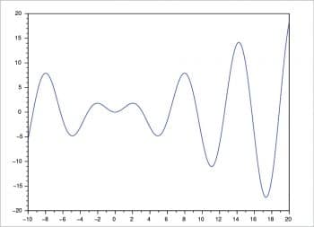
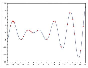
To feel the power of Scilab, let’s implement a swarm intelligence based algorithm in it. Note that we use a single variable for ease of visualisation. The function f (x) = x sin(x) has a single variable x, and we want to find the value for x such that the function is minimum. Essentially, the above example is a minimisation problem, and these kinds of problems come under optimisation. If we plot the function for variable x, by looking into the function plot, we can infer that the minimum value lies somewhere between 17 and 18. To find it with the fire-fly algorithm, we have the help of 25 fire-flies. We scatter the flies along the function, so that we have flies in different locations along the function plot. The brightness of the flashes given out by each fly increases with its proximity to the exact location of the solution. The equation governing this process is:
<em>x<sub>i</sub> = x<sub>i</sub> + β<sub>j</sub> x e<sup>rx—r2</sup><sub>ij</sub> x (x<sub>j</sub> — x<sub>i</sub>) + αЄ<sub>i</sub></em>
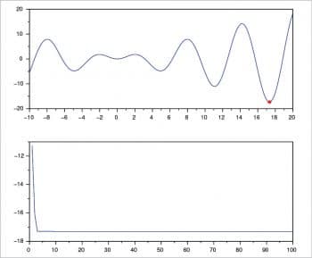
After 100 iterations, the result obtained is 17.307. This is shown with the convergence, as seen in Figures 1, 2 and 3. Hence, we have seen the action of the fire-fly algorithm in finding the minimum, using Scilab.
Engineering problems, which are more like real world problems, tend to be highly non-linear in nature. They can be easily tackled with evolutionary methods like this. Unfortunately, Scilab is mostly ignored by academia, and its power is often overlooked.


