Julia is a rising star in the world of programming languages, having inherited the best features of both Python and C. This article provides insights into the machine learning related features offered by Julia. As it is optimised for both speed and ease-of-use, developing machine learning based applications in Julia is fairly straightforward.
The world of programming languages always faces the conundrum of selecting a language from two variants – one that is easy to use and another that produces optimal code. For example, a language like Python is very easy to use but has a sub-optimal performance with respect to speed. And languages like C, which produce near-optimal code, are taxing on programmers. Julia is a perfect combination of both these worlds. If you are new to Julia, you might prefer to read an article in an earlier issue of Open Source For You titled, ‘Julia: A Language that Walks like Python and Runs like C’. In addition to this, there are plenty of resources on the Web that enable a developer to become familiar with Julia (http://docs.julialang.org/en/release-0.5/).
The focus of this article is to introduce readers to machine learning and associated tasks in Julia. The core idea of machine learning is to enable machines to model the problem space in such a way that programs are capable of handling novel scenarios. For example, an artificial neural network for digit recognition should be able to recognise the variations of digits that were not present in the training dataset. In simple words, these networks are bio-inspired, similar to the manner in which biological creatures respond to scenarios, after successful training. Machine learning can be used across various domains such as text recognition, image recognition, classification, etc.
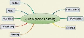
Similar to Python, Julia is also extensible. It has many libraries and packages focusing on specific domains. For machine learning itself, Julia has various libraries, as shown in Figure 1.
This article provides an introduction to a few of these libraries.
ScikitLearn.jl
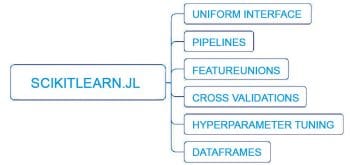
Julia has a library called ScikitLearn.jl. This library is aimed towards bringing the features of scikit-learn python library to Julia. Scikit-learn, which is very popular with Python developers involved in machine learning based projects and has implemented the scikit-learn algorithms. The major features of ScikitLearn.jl are listed below:
- It has around 150 models accessed with a uniform interface
- Pipelines and FeatureUnions
- Cross-validation
- Hyperparameter tuning
- DataFrames support
Installation of ScikitLearn.jl may be done using the following command:
Pkg.add(“ScikitLearn”)
It has to be noted that the scikit-learn Python library is required to import the optional Python modules. Pyplot.jl is also utilised. As noted in the official documentation, ScikitLearn.jl is not associated with scikit-learn.org.
A simple classifier example with the Iris dataset and LogisticRegression is shown below (http://scikitlearnjl.readthedocs.io/en/latest/quickstart/):
# The Rdataset shall be added, if unavailable.
using RDatasets: dataset

iris = dataset(“datasets”, “iris”)
# ScikitLearn.jl expects arrays, but DataFrames can also be used - see
# the corresponding section of the manual
X = convert(Array, iris[[:SepalLength, :SepalWidth, :PetalLength, :PetalWidth]])
y = convert(Array, iris[:Species])

# Load the Logistic Regression model
using ScikitLearn
# This model requires scikit-learn. See
# http://scikitlearnjl.readthedocs.io/en/latest/models/#installation
@sk_import linear_model: LogisticRegression
# The Hyperparameters such as regression strength, whether to fit the intercept, penalty type.
model = LogisticRegression(fit_intercept=true)

# Train the model.
fit!(model, X, y)

# Accuracy is evaluated
accuracy = sum(predict(model, X) .== y) / length(y)
println(“accuracy: $accuracy”)
The cross-validation is shown in the code given below:
using ScikitLearn.CrossValidation: cross_val_score

cross_val_score(LogisticRegression(), X, y; cv=5)  # 5-fold
> 5-element Array{Float64,1}:
>  1.0
>  0.966667
>  0.933333
>  0.9
>  1.0
ScikitLearn.jl may be used with other classifiers such as the DecisionTree classifier (DecisionTree.jl – https://github.com/bensadeghi/DecisionTree.jl). A random Forest based classifier is also shown below:
using RDatasets: dataset
using DecisionTree
iris = dataset(“datasets”, “iris”)
features = convert(Array, iris[:, 1:4]);
labels = convert(Array, iris[:, 5]);

# train full-tree classifier
model = DecisionTreeClassifier(pruning_purity_threshold=0.9, maxdepth=6)
fit!(model, features, labels)
# pretty print of the tree, to a depth of 5 nodes (optional)
print_tree(model.root, 5)
# apply learned model
predict(model, [5.9,3.0,5.1,1.9])
# get the probability of each label
predict_proba(model, [5.9,3.0,5.1,1.9])
println(get_classes(model)) # returns the ordering of the columns in predict_proba’s output
# run n-fold cross validation over 3 CV folds
# See ScikitLearn.jl for installation instructions
using ScikitLearn.CrossValidation: cross_val_score
accuracy = cross_val_score(model, features, labels, cv=3)
The following models are available in DecisionTree.jl:
- DecisionTreeClassifier
- DecisionTreeRegressor
- RandomForestClassifier
- RandomForestRegressor
- AdaBoostStumpClassifier
TensorFlow
TensorFlow is a recent buzzword in the machine learning world. This active open source machine learning framework from Google focuses on numerical computation with data flow graphs. The nodes represent mathematical operations, and the edges connecting the node indicate the data arrays termed Tensors. TensorFlow.jl is a Julia wrapper for TensorFlow, which can be installed using Pkg.add, as shown below:
Pkg.add(“TensorFlow”)
Using the GPU for efficient processing is an important attribute of machine learning approaches. To activate the GPU support, the environment variable TF_USE_GPU needs to be set to 1. To enable GPU usage, CUDA 7.5 and cudnn are needed.
ENV[“TF_USE_GPU”] = “1”
Pkg.build(“TensorFlow”)
It has to be noted that the TensorFlow API is huge, and all the functionalities are not wrapped at present. Some of the currently available functionalities are listed below:
- Unary and binary mathematical functions
- Commonly used neural network operations. This covers convolutions, recurrent neural networks, etc
- Fundamental image-loading and resizing operations
The following are not currently wrapped:
- Control flow operations
- Distributed graph execution
- PyBoard graph visualisation
A code fragment to classify MNIST digits with TensorFlow is provided in this section (https://malmaud.github.io/tfdocs/tutorial/).
1. The TensorFlow session is built as shown below:
using TensorFlow
sess = Session()
2. A Softmax Regression Model is built as follows:
x = placeholder(Float32)
y = placeholder(Float32)
W = Variable(zeros([784, 10]))
b = Variable(zeros([10]))
run(sess, initialize_all_variables())
y = nn.softmax(x*W + b)
cross_entropy = reduce_mean(-reduce_sum(y_ .* log(y), reduction_indices=[2]))
3. Training of the model is shown below:
train_step = train.minimize(train.GradientDescentOptimizer(.00001), cross_entropy)
for i in 1:1000
    batch = next_batch(loader, 100)
    run(sess, train_step, Dict(x=>batch[1], y_=>batch[2]))
end
4. The model evaluation is done using the following code snippet:
correct_prediction = indmax(y, 2) .== indmax(y_, 2)
accuracy=reduce_mean(cast(correct_prediction, Float32))
testx, testy = load_test_set()

println(run(sess, accuracy, Dict(x=>testx, y_=>testy)))
MXNet
MXNet is an active deep learning package available in Julia. It facilitates efficient GPU handling for optimal results. MXNet.jl is the Julia version of dmlc/mxnet (https://github.com/dmlc/mxnet). The major features of MXNet.jl are:
- It enables efficient tensor computation; it can efficiently handle multiple computing devices, GPUs and distributed nodes.
- It facilitates effective manipulation of deep learning models.
- A simple three-layer MLP can be defined as follows:
using MXNet
data = mx.Variable(:data)

fc1  = mx.FullyConnected(data = data, name=:fc1, num_hidden=128)
act1 = mx.Activation(data = fc1, name=:relu1, act_type=:relu)
fc2  = mx.FullyConnected(data = act1, name=:fc2, num_hidden=64)
act2 = mx.Activation(data = fc2, name=:relu2, act_type=:relu)
fc3  = mx.FullyConnected(data = act2, name=:fc3, num_hidden=10)
The aforementioned code fragment forms a feedforward chain. The recognition of digits 0 to 9 is handled with 10 output classes. A complete tutorial sequence is available at http://dmlc.ml/MXNet.jl/latest/tutorial/mnist/#Convolutional-Neural-Networks-1.
Machine learning incorporates a large spectrum of approaches. This article is just the tip of the iceberg. If you are interested in learning more about the topic, then the following link has pointers to plenty of resources in one place: https://github.com/josephmisiti/awesome-machine-learning.


