Programming in R

R is a language and environment for statistical computing and graphics. It is a simple and effective programming language, which includes conditionals and loops. Often called GNU S, it is used to statistically explore datasets and to make many graphical displays of data.

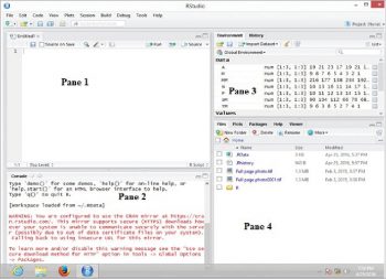
R is a highly powerful computer language, an environment and integrated suite of software facilities. The functionality of R can be easily extended via packages. A typical R studio window might have four panes as depicted in Figure 1.

The user can type the commands in Pane 1 and press Ctrl + Enter in order to execute the entered command. The output will appear in Pane 2, i.e., the pane with the caption ‘Console’. Alternatively, the user might type the command in the Console pane itself and obtain the result on pressing the Enter key.

This section dwells on the following: accepting input from the keyboard, generating sequences, and random numbers in R.

scan() can be used for obtaining numeric inputs from the keyboard, as shown below:

> x2 <- scan()

Now the user can enter the numbers in the Console window and press the Enter key instead of entering a number in order to indicate the end of data input.  The numbers will be assigned to x2.

Sequence-generating operator

The colon (:) can be used to generate sequences in R, as follows:

> x <- 11:20     # the integers in the range 11 to 20 (both inclusive) will be
        # stored  in x
> x        # print the values stored in x

For shuffling the values stored in x, the sample() function can be used:

> q<-sample(x)
> q

The values stored in q might be: 13 14 16 19 17 15 12 11 18 20. The values stored in x remain intact.

seq() can be used in R for generating a sequence, as follows:

> z <- seq(from=11,to=30,by=3)
> z

A sample output follows:

[1] 11 14 17 20 23 26 29

In Figure 1, the command from is for specifying the starting value of the sequence, to is for specifying the ending value of the sequence, and by is to increment the sequence.
The concatenation function can be used to store values in x1, as shown below:

> x1 <- c(11,12,13,14,15,16,17,18,19,20)     
                        #assigning integers in the range  
                           #11 to 20
> x1                           #print the values stored in x1

Random numbers in R
Random numbers are used in simulation and they are also used by statisticians.
To generate a random number (having a fractional part) between 11 and 15, and store it in rnum, the following command can be used:

> rnum <- runif(1,11,15)
> rnum        # print the value of rnum
[1] 14.75596 (Sample output)

By default, runif(n) generates random numbers in the range of 0 to 1.

> rnum <- runif(10,11,15)     # for generating 10 random numbers     # in the range of 11 to 15

In order to generate three integer random numbers between 11 and 15, the following command can be used:

> x <- sample(11:15,3,replace=T)
> x

11:15 is the range between which random numbers have to be generated, 3 the number of random numbers to be generated and replace = T, which indicates that repeats are permissible.

For generating a sequence of random numbers, and to generate the same sequence later, set.seed() and runif() can be used as follows:

> set.seed(7)
> runif(7)

Note: 1) Help is readily available in R. In order to obtain help on random numbers, the following command might be helpful:

help.search(“random numbers”)

2) <- (Less than, followed by the minus symbol) is the assignment operator in R. Alternatively, the ‘=’ operator can also be used.
3) R is a case-sensitive language.

The section below dwells on vector and matrix operations in R.

Vectors in R
The R programming environment provides very powerful vector and matrix operation tools. The code below creates a vector for storing the first 13 members of the Fibonacci series:

Code snippet 1
> fib <- numeric(13)

> fib[1] <- 0
> fib[2] <- 1
> for(idx in 3:13) {
+   fib[idx] <- fib[idx-1] + fib[idx - 2]
+ }
> fib

The output of the above code would be:

 [output]   0   1   1   2   3   5   8  13  21  34  55  89 144

 

• fib <- numeric(13): Sets up a numeric vector the length of which is 13 and this vector is initialised with zeroes.
• fib[1] <- 0: Sets the first element of vector fib to the value 0. The next statement is self-explanatory.
• The for() loop computes the third to the thirteenth element  (except for the first two elements, each term in the Fibonacci series is the sum of the preceding two terms).
• fib: Displays the elements of the vector fib.

The contents of the fib vector can also be printed with the help of the for() loop, as shown below:

> for(idx in 1:13)
+   print(fib[idx])

A sample output is shown below:

0
1
1
2
3
5
8
13
21
34
55
89
144

is.vector(x) and is.matrix(x) can be used to determine whether x is a vector or matrix.
> is.vector(fib) will yield the following:

[output] TRUE

And > is.matrix(fib) will yield what follows:

[output] FALSE

A few more commands (along with the output) related to vector operations are as follows:

> min(fib)    #for finding minimum value in a vector
[output] 0
> max(fib)     #for finding maximum value in a vector
[output] 144
> mean(fib)     #for finding mean value
[output] 28.92308
> median(fib)     #for finding median value
[output] 8
> var(fib)     #for finding variance
[output] 1889.744
> sd(fib)     #for finding standard deviation
[output] 43.47118
> sort(fib,decreasing = TRUE)     #for sorting in descending order
[output] 144  89  55  34  21  13   8   5   3   2   1   1   0
> sum(fib)     #for finding sum of the vector elements
> summary(fib)
Min. 1st Qu.  Median    Mean 3rd Qu.    Max.
0.00    2.00    8.00   28.92   34.00  144.00

Matrix operations in R
This part of the article dwells on the terseness of complex matrix operations in R.
The command…

M <- matrix(c(9,8,7,6,5,4,3,2,1),3,3)

…creates a 3 x 3 matrix as follows:

[,1] [,2] [,3]
[1,]    9    6    3
[2,]    8    5    2
[3,]    7    4    1

Note: 1) [2,] refers to the second row and [,3] refers to the third column.
2) The numbers are, by default, entered into the matrix in a column-wise fashion.

The command…

N <- matrix(c(10,11,12,13,14,15,16,17,18), 3, 3,byrow=TRUE)

…creates a 3 x 3 matrix as follows:

[,1] [,2] [,3]
[1,]   10   11   12
[2,]   13   14   15
[3,]   16   17   18

In order to display matrix M, the user can simply type the following command…

M

…at the ‘>’ prompt and press Ctrl + Enter.

For adding matrices M and N, and storing the result in matrix A, the user can type the following commands:

> A <- M + N
> A

The output will appear as follows:

[,1] [,2] [,3]
[1,]   19   17   15
[2,]   21   19   17
[3,]   23   21   19

In order to store the transpose of M into TM and for displaying TM, the following commands can be used:

> TM <- t(M)
> TM
[,1] [,2] [,3]
[1,]    9    8    7
[2,]    6    5    4
[3,]    3    2    1

To multiply matrices M and N and store the result in matrix MM, the following commands can be used:

> MM <- M %*% N
> MM
[,1] [,2] [,3]
[1,]  216  234  252
[2,]  177  192  207
[3,]  138  150  162

Note: The system won’t crash if the matrices are not conformable for multiplication.

If the commands typed are…

<em>&gt; SM &lt;- M * N</em>
<em>&gt; SM</em>

…then the output will be:

To find the determinant of M and display the result, use the following commands:

> d <- det(M)
> d

To find the inverse of matrix M, use the following command:

> MI <- solve(M)

To find the rank of matrix M, type in the following command:

rm <- qr(M)
> rm

A typical output is shown below:

$qr
[,1]       [,2]          [,3]
[1,] -13.9283883 -8.7590895 -3.589791e+00
[2,]   0.5743665  0.5275893  1.055179e+00
[3,]   0.5025707  0.9589395  1.280443e-16
$rank
[1] 2
$qraux
[1] 1.646162e+00 1.283611e+00 1.280443e-16
$pivot
[1] 1 2 3
attr(,”class”)
[1] “qr”

For combining matrices M and N (columnwise), use the following command:

> cbind(M,N)

The output will be as follows:

[,1] [,2] [,3] [,4] [,5] [,6]
[1,]    9    6    3   10   11   12
[2,]    8    5    2   13   14   15
[3,]    7    4    1   16   17   18

For combining matrices M and N (row wise), use the following command:

> rbind(M,N).

Note: 1) To get a list of all the variables that have been defined in a R session, use the ls() command.

2) To display the warnings being generated by a code snippet, use warnings().
3) To exit from R, use q().

Pie charts in R
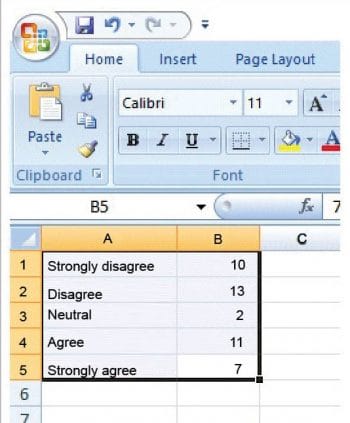
Assume that a csv file (C:\Users\faculty\Documents\info.csv) contains the  data given in Figure 3.
A pie chart can be drawn based on the data in Figure 3, with the following commands:

> d<- read.csv(“C:/Users/faculty/Documents/info.csv”,header=FALSE,sep=”,”)
# for assigning the data in the file info.csv to d
> d # for displaying the value of d

R automatically assigns names to the rows and columns. The row names and column names can be displayed using the following commands:

> rownames(d)
[sample output] “1” “2” “3” “4” “5”
> colnames(d)
[sample output] “V1” “V2”

To display the values of V1 and V2, the following commands can be used:

> d$V1
{Sample output:
[1] Strongly disagree Disagree          Neutral
[4] Agree             Strongly agree
5 Levels: Agree Disagree Neutral ... Strongly disagree
> d$V2
[1] 10 13  2 11  7}
> lab<- round(d$V2/sum(d$V2) * 100,1)
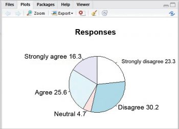
> pie(d$V2,labels=paste(d$V1,lab, sep = “ “),main=”Responses”,clockwise=TRUE)

A pie chart will appear in the Plots window as shown in Figure 4.
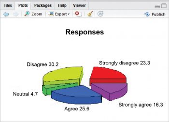
pie3D() can be used for generating a 3D pie chart. To use pie3D(), it is necessary to install the plotrix package:

> install.packages(“plotrix”)
> library(plotrix)
> pie3D(d$V2,labels=paste(d$V1,lab, sep = “ “),main=”Responses”,explode=0.2)

R language can be used to perform highly complex operations related to statistics as well as econometrics. It can also be used for working on images and mathematical modelling. In fact, many premier institutions in several countries have made R a part of their regular curriculum, and insist on researchers using this language for carrying out statistical research.