Get Analytical with R

With a spreadsheet, some types of calculations are difficult to carry out. So I was on the look out for software to complement the spreadsheet. This software had to be free (as in freedom and, if possible, as in beer) and open source, powerful, lightweight, fast, used by many people, very well documented and easy to learn. All these features in one software seemed almost impossible to find. Yet, after a search, I found ‘R’. Since the full code of each example presented here is too long for a magazine article, it’s freely available at https://github.com/astonfe/r

Potentiometric titration
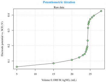
Titration is a common laboratory method of quantitative chemical analysis that is used to determine the unknown concentration of an identified analyte. This experiment is taken from Reference 3 given at the end of the article, and is about the potentiometric titration curve for 2.433 meq of Cl- with 0.1000 M AgNO3. The raw data are read from an xls file (LibreOffice Calc) via the gdata package, which requires the Perl language to be installed on the computer. This is not a particular problem under GNU Linux, but Strawberry Perl (http://strawberryperl.com) must be installed if you’re using Windows. This is not the only way, though. There are other options to read xls files from R. The raw data (Figure 1) can be easily plotted with the use of the following code:

plot(x,y,type=”n”)
grid(...)
points(x,y,type=”o”)

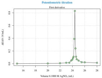
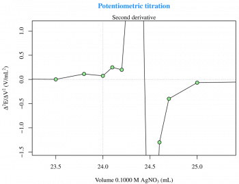
The first and the second derivatives (Figures 2 and 3) are useful to determine the inflection point. The derivatives can be calculated with two for loops and then plotted as previously seen for the raw data, as follows:

f=vector()
for(i in 2:n) {
f[[i]]=((y[[i]]-y[[i-1]])/(x[[i]]-x[[i-1]]))
}
x1=x[2:n,drop=T]
y1=f[2:n,drop=T]
plot(x1,y1,type=”n”)
grid(...)
points(x1,y1,type=”o”)
s=vector()
for(i in 3:n) {
s[[i]]=((f[[i]]-f[[i-1]])/(x[[i]]-x[[i-1]]))
}
x2=x[3:n,drop=T]
y2=s[3:n,drop=T]
plot(x2,y2,type=”n”)
grid(...)
points(x2,y2,type=”o”)

Now, with a zm(type=”session”), I can zoom on the plot (Figure 3) for a better visualisation and then, with locator(), I can obtain the inflection point coordinates.

Conductometric titration
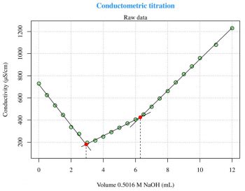
For a general explanation of this technique, log on to http://en.wikipedia.org/wiki/Conductometry. The first experiment (Figure 4) is taken from Reference 5 given at the end of the article and is about the conductometric titration curve for NaOH with 0.1219 M potassium hydrogen phthalate (C8H5KO4). The second experiment (Figure 5) is also taken from the same reference, and is about the conductometric titration curve for H3PO4 with 0.5016 M NaOH. These two experiments are problems of linear segmented regression (see Reference 6) about the determination of the break-point(s). The most important aspect relates to the psi parameter within the segmented package call. The psi parameter includes starting values for the break-point(s) for the corresponding variable in seg.Z. If seg.Z includes only a variable, psi may be a numeric vector. With summary(fit) I can visualise the break-point(s) coordinates on the x axis. The easiest way to plot the regression lines is the use of abline(intercept,slope,col=your-color), but the abline line type spans the whole plot width. The figures presented here have been arrived at with some more calculations and the regression lines are plotted with lines. The following code can be used to calculate the slope and the intercept for each segment:

fit<-segmented(lm(y~x),seg.Z=~x,psi=list(x=c(5))) # Figure 4
a1=slope(fit)$x[1]
b1=intercept(fit)$x[1]
...
fit<-segmented(lm(y~x),seg.Z=~x,psi=list(x=c(3,6))) # Figure 5
a1=slope(fit)$x[1]
b1=intercept(fit)$x[1]
...

Let me add something about the use of the Greek letters. Look at the following two examples:

ylab=expression(“Conductivity (“*mu*”S/cm)”)
ylab=expression(“Conductivity ( “*mu*”S/cm)”)

The first is preferable if the plot will be exported to PDF and the second, if a space is added after “(”, if it is in PNG. With some limitations, it’s also possible to directly use the ‘micro’ symbol, but probably the best thing is to use the unicode string “\u00b5”. I think that the use of a more general technique could be better than this.

Linear fit weighted and printed with Markdown
A weighted model is very widely used in some applications (for example, in pharmacokinetics studies). With a few lines of code I can define all the models I need. The most important aspect of this topic is the calculation of the percentage accuracy for the back-calculated concentrations, as reported in the following code:

# fit<-lm(y~x) # Linear fit simple
fit<-lm(y~x,weight=1/x^2) # Linear fit weighted
a=coef(fit)[2]
b=coef(fit)[1]
# fit<-lm(y~0+x) # Linear fit through origin
# a=coef(fit)[1]
# b=0
summary(fit)$coef
Predicted=(y-b)/a
Accuracy=(Predicted*100)/x
cbind(data,Predicted,Accuracy)

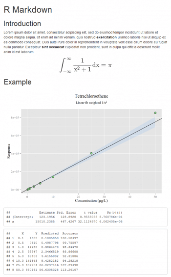
The table that is made with cbind, in which the data is present, the x values back-calculated (usually the concentration is reported on the x axis) and its percentage accuracy, are all very useful. For more theory, see Reference 7 given at the end of the article. Printing a notebook-like document is possible with the R Markdown package (though other options exist). Generally speaking, using my preferred text editor, I can write a document called, for instance, example.Rmd which contains text and code; then R is used as a compiler only. If Pandoc (http://www.pandoc.org) is installed, typing rmarkdown::render(“example.Rmd”) from the R console, produces the HTML file with the text formatted according to the Markdown syntax, a plot and the results of some calculations (Figure 6). It’s very easy, so issue the following commands:

# Title

## Section 1

$$your-mathematical-formula$$

## Section 2

```{r,message=F,echo=F}
...
ggplot(data.frame(x=x,y=y),aes(x=x,y=y))+
geom_ribbon(aes(y=p[,”fit”],ymin=p[,”lwr”],ymax=p[,”upr”],fill=”confidence”),alpha=0.1)+
scale_fill_manual(values=”#1E90FF”)+
geom_point(shape=21,col=”black”,fill=”#90EE90”,size=3)+
geom_abline(slope=a,intercept=b)+
labs(x=”Concentration (µg/L)”,y=”Response”)+
ggtitle(expression(atop(“Tetrachloroethene”,atop(“Linear fit weighted 1/x”^2))))+
theme(legend.position=”none”)
...
```

The plot is built with ggplot and the confidence band is added. In this example, the options message (to display R messages) and echo (to display the code along with its results) are set to ‘False’. More complex documents can be produced according to http://rmarkdown.rstudio.com.

Emacs Speaks Statistics
With Emacs Speaks Statistics (http://ess.r-project.org), the user can edit R language commands in one GNU Emacs buffer and execute the code in a second (see Reference 9). Under Windows, an interesting way to do this is to use the GNU Emacs distribution prepared by Professor Vincent Goulet (Université Laval) and this is available for Mac OS too (http://vgoulet.act.ulaval.ca/en/emacs). I’m not an enthusiast of ESS because I think there’s an interesting approach under GNU Linux but, when I’m using Windows, R has its own script editor and ‘Edit > Run all’ works fine for me.
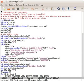
There’s another problem related to highlighting syntax. By default, the R language is poorly supported by Vim and not supported by GNU Emacs. The package ESS adds some syntax highlighting support to GNU Emacs for the R language. I’m not very satisfied with it because all the keywords have the same colour (Figure 7). This is probably due to the R keywords not being categorised. To have more effective syntax highlighting, I think it will be necessary to organise the keywords better, perhaps in a manner similar to Scilab (see OSFY, June 2015). Practically, it’s not necessary to classify all the keywords (which could run into thousands) but only the keywords I’m using (200, more or less). For example, I can have different groups/colours for keywords about statistics (lm, coef, predict …), plotting (plot, points, abline …), ggplot (ggplot, geom_something, ggtitle …), generic (cbind, par, summary …) and more. This is more or less the same as in a ‘human-spoken’ language: it has a vocabulary (the keywords) with which it is possible to find various categories such as substantives, adjectives, verbs, adverbs, etc. Using this classification, I can build a syntax highlighting a file for Vim, GNU Emacs, jEdit, Notepad++, etc. An interesting explanation of ESS is written by Rodney Sparapani as reported in Reference 10.

There’s one more thing that must be said about the file encryption. Usually, my R files are not encrypted, but if a backup is done on a remote server, I prefer to encrypt them using GPG (GNU Privacy Guard, http://www.gpg4win.org). Yes, under Windows, because in my work experience I have encountered only one company that uses GNU Linux as a desktop system.
First, it’s necessary to generate my key using GPA (GNU Privacy Assistant). Now Emacs can interact directly with GPG. In Emacs, visit a new file with a .gpg extension. For example, my-script.R.gpg and then place this line at the top of the file: # -*- epa-file-encrypt-to: (“your@email.address”) -*- When you try to save the file, Emacs will show a prompt in a buffer under it. Move the cursor to the line containing the key and hit ‘m’. Move the cursor to ‘OK’ and hit ‘<return>’. Next time, when I open that .gpg file, I will be prompted for the password only once and then consecutive saves will be password-prompt-free. More details can be found on Emacs Stack Exchange (see Reference 11).
Without fear of contradiction, it can be said that R is today the lingua franca of statistics. In my opinion, it’s one of the best examples of FOSS. The titration examples presented here are a bit unusual for an IT magazine, but do consider the fact that the automatic detection of one or more break-points in conductometric titrations is very useful in daily practice. I don’t know if there are other free and open source software that do this as well as the segmented package for R.
R is also very well documented. There are a lot websites and books available to discover new things about it.

References
[1] http://en.wikipedia.org/wiki/Titration, last visited on 04/07/2015.
[2] http://en.wikipedia.org/wiki/Potentiometric_titration, last visited on 04/07/2015.
[3] Skoog, Principles of instrumental analysis, Saunders, Philadephia, 1985.
[4] http://en.wikipedia.org/wiki/Conductometry, last visited on 04/07/2015.
[5] Cozzi, Protti, Ruaro, Analisi chimica strumentale, Metodi elettrochimici (Instrumental analytical chemistry, Electrochemical methods), Zanichelli, Bologna, 1997.
[6] http://en.wikipedia.org/wiki/Segmented_regression, last visited on 04/07/2015.
[7] Massart, Vandeginste, Buydens, De Jong, Lewi, Smeyers-Verbeke, Handbook of chemometrics and qualimetrics, Elsevier, Amsterdam, 2003.
[8] http://rmarkdown.rstudio.com, last visited on 04/07/2015.
[9] http://en.wikipedia.org/wiki/Emacs_Speaks_Statistics, last visited on 04/07/2015.
[10] http://blog.revolutionanalytics.com/2014/03/emacs-ess-and-r-for-zombies.html, last visited on 04/07/2015.
[11] http://emacs.stackexchange.com/questions/12212, last visited on 04/07/2015.