Building Image Processing Embedded Systems using Python, Part 2

As I had mentioned in the previous article, OpenCV is a very powerful library that is used for image processing. I will now explain its syntax and how to use it, along with a few examples. I will not go into the basics of Python code and syntax, since this is extensively documented.

Reading and displaying an image

Our first example, which I have named Test.py‘ is short:

#!/usr/bin/python
import cv
src = cv.LoadImage("/home/jayneil/12.png")
cv.NamedWindow("RGB",cv.CV_WINDOW_AUTOSIZE)
cv.ShowImage("RGB", src)
cv.WaitKey(500)
cv.DestroyWindow("RGB")

In a terminal, navigate to the directory that contains the file, and run it with python Test.py. The output can be seen in Figure 1 — our image in a window.

Import the OpenCV module cv so that you can use it, then call the LoadImage function (passing the full path to the file, which is needed) to load the image into the variable src. The NamedWindow function creates a window in which to display the loaded image. The first parameter is the name for the window, and the second sets the sizing mode to automatically resize the window to the size of the image.

Next, ShowImage is used to display the image in the window, passing it the name of the window and the image variable. After that, WaitKey is used so that you can see the image for a sizeable period of time (similar to a delay function). Finally, DestroyWindow destroys the window and frees the resources it used.

Converting an RGB image to grey-scale format

Most digital images seen in everyday life use the RGB colour model, in which every pixel has three components — red, green and blue. By varying the amount of each component, a pixel gets a unique colour. Grey-scale is another popular colour model, with only one component, which varies from 0-255; 0 represents black, and 255 white (for an 8-bit image). The code below, Rgb2gray.py, converts an image from RGB to grey-scale:

#!/usr/bin/python
import cv
src = cv.LoadImage("/home/jayneil/12.png")
cv.NamedWindow("RGB", cv.CV_WINDOW_AUTOSIZE)
cv.ShowImage("RGB", src)
cv.WaitKey(500)
cv.DestroyWindow("RGB")
dst = cv.CreateImage(cv.GetSize(src), cv.IPL_DEPTH_8U, 1)
cv.CvtColor(src, dst, cv.CV_RGB2GRAY)
cv.NamedWindow("GRAY", cv.CV_WINDOW_AUTOSIZE)
cv.ShowImage("GRAY", dst)
cv.WaitKey(1000)
cv.DestroyWindow("GRAY")

Running this should result in output similar to Figure 2.

I’ll skip the functions I’ve already explained. In the eighth line, we have created our own image, similar to the source image (src). GetSize returns the properties of the source image — so our new image has the same dimensions as the source. CreateImage takes three parameters: the image dimensions, the colour depth of the image (8-bit or 16-bit) and the number of channels (which, for grey-scale, is one).

We used the CvtColor function to convert the image to grey-scale. This function has three parameters. The first one is the name of the image which we want to convert and the second denotes what type of conversion we want to do. The third parameter performs the type of conversion desired. In this case it is from RGB to grey-scale.

Drawing a circle on an image

You can also edit or manipulate a given image, for example, like drawing a circle on it. The following code (Circle.py) does this:

#!/usr/bin/python
import cv
src = cv.LoadImage("/home/jayneil/12.png")
print(src)
cv.NamedWindow("RGB", cv.CV_WINDOW_AUTOSIZE)
cv.ShowImage("RGB", src)
cv.WaitKey(1000)
cv.DestroyWindow("RGB")
thickness = 3
lineType=8
Point = (292,300)
cv.Circle(src, Point,100, cv.Scalar(0,0,255), thickness, lineType)
cv.NamedWindow("Circle_on_image", cv.CV_WINDOW_AUTOSIZE)
cv.ShowImage("Circle_on_image", src)
cv.WaitKey(3000)
cv.DestroyWindow("RGB")

Run it. The output should resemble Figure 3.

From the ninth to the 11th line, we have described the parameters of the circle — its thickness, line type and coordinates. On Line 12, the Circle function is used, which has six parameters: the target image on which to draw the circle, the coordinates, the radius of the circle, the colour of the circle, the thickness and the line type. Other code is similar to previous examples.

The Laplacian of an image

Often, the Laplace operation is performed on an image to get the edges. The code below (Laplace.py) does this:

#!/usr/bin/python
import cv
src = cv.LoadImage("/home/jayneil/12.png")
print(src)
cv.NamedWindow("RGB", cv.CV_WINDOW_AUTOSIZE)
cv.ShowImage("RGB", src)
cv.WaitKey(1000)
cv.DestroyWindow("RGB")
dst = cv.CreateImage(cv.GetSize(src), cv.IPL_DEPTH_16S, 3)
laplace = cv.Laplace(src, dst)
cv.SaveImage("/home/jayneil/laplace.png", dst)
temp=cv.LoadImage("/home/jayneil/laplace.png")
cv.NamedWindow("Laplace", cv.CV_WINDOW_AUTOSIZE)
cv.ShowImage("Laplace", temp)
cv.WaitKey(2000)
cv.DestroyWindow("Laplace")

Figure 4 shows the expected output of running the code given above.

The print function outputs the properties of the image. On the 10th line, the laplace function is used to obtain the edges. It takes two parameters — the source image and the variable in which to store the processed image. You can use SaveImage to save the resultant image, supplying the path, the file name, and the variable containing the image. Then load the saved image and display it.

The Canny filter

This is a very popular filter, used to very accurately detect the edges in an image. The code below is Canny.py:

#!/usr/bin/python
import cv
src = cv.LoadImage("/home/jayneil/12.png")
cv.NamedWindow("RGB", cv.CV_WINDOW_AUTOSIZE)
cv.ShowImage("RGB", src)
cv.WaitKey(1000)
cv.DestroyWindow("RGB")
dst = cv.CreateImage(cv.GetSize(src), cv.IPL_DEPTH_8U, 1)
cv.CvtColor(src, dst, cv.CV_RGB2GRAY)
cv.NamedWindow("GRAY", cv.CV_WINDOW_AUTOSIZE)
cv.ShowImage("GRAY", dst)
cv.WaitKey(1000)
cv.DestroyWindow("GRAY")
dst1 = cv.CreateImage(cv.GetSize(src), cv.IPL_DEPTH_8U, 1)
cv.Canny(dst, dst1, 1.0, 4.0, aperture_size=3)
cv.NamedWindow("Canny_Filter", cv.CV_WINDOW_AUTOSIZE)
cv.ShowImage("Canny_Filter", dst1)
cv.WaitKey(4500)
cv.DestroyWindow("Canny_Filter")

Run the code and you should see something like what’s shown in Figure 5.

Convert the input image to grey-scale first (see the ninth line), before applying the canny filter in the 15th line. This function takes five parameters: the source image, the variable in which to store the processed image, and the rest are the threshold values for this filter.

Face detection

Finally, let us detect faces in a still image, using a Haar classifier for detection. The Haar classifier is a pre-made program, which you can train to do operations based on your needs. The more you run the program, the more the Haar classifier trains itself. All Haar classifiers are located in OpenCV-2.3.0/data/haarcascades. The following is Face.py:

#!/usr/bin/python
import cv  #import the openCV lib to python
a=cv.LoadImage("/home/jayneil/beautiful-faces.jpg")
print(a)
cv.NamedWindow("Original Image", cv.CV_WINDOW_AUTOSIZE)
cv.ShowImage("Original Image", a)
cv.WaitKey(6000)
cv.DestroyWindow("Original Image")
hc = cv.Load("/home/jayneil/haarcascade_frontalface_default.xml")
img = cv.LoadImage("/home/jayneil/beautiful-faces.jpg", 0)
faces = cv.HaarDetectObjects(img, hc, cv.CreateMemStorage())
for (x, y, w, h), n in faces:
    cv.Rectangle(img, (x, y), (x+w, y+h), 255)
cv.SaveImage("faces_detected.jpg", img)
print(faces)
dst=cv.LoadImage("faces_detected.jpg")
cv.NamedWindow("Face Detected", cv.CV_WINDOW_AUTOSIZE)
cv.ShowImage("Face Detected", dst)
cv.WaitKey(5000)
cv.DestroyWindow("Face Detected")

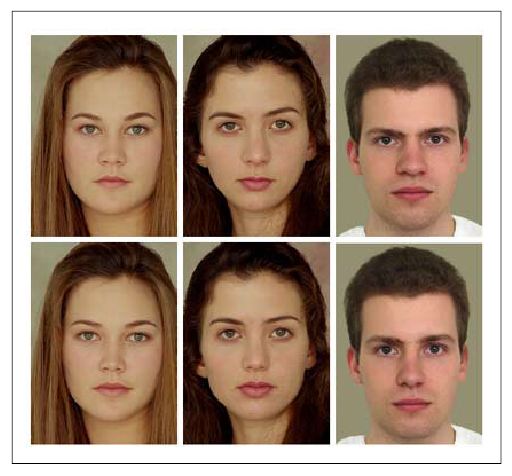
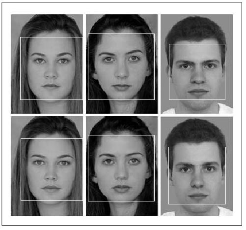
Run the code. The source image I used is shown in Figure 6, and the output in Figure 7.

In the ninth line, I have stored the Haar classifier that I want to use, in a variable. In the 11th line, I have used the HaarDetectObjects function to detect the features I want. This function has three parameters. The first one is the source image, the second the Haar classifier I want to use and the third one creates a memory storage. Then I have used a for loop to draw a rectangle around the portion that I have identified in the previous stage, using the Rectangle function, which takes four parameters: the image on which to draw, followed by the two opposite corners of the rectangle, and the last one denotes the colour.

In the third and final part of the series, I will cover how to program and use the Arduino. I will also cover how to use the Pyserial module and how to integrate all the technologies we have learned so far to build an embedded system for image processing.

Please refer to the OpenCV documentation for more information.