


Some of our readers have requested me to cover neural networks. This topic has attracted a lot of interest and attention lately.
While neural networks can be applied to different applications such as image recognition and speech processing, we will discuss neural networks with a focus on natural language processing. Let’s start off with a quick overview of the application of neural networks in natural language processing.
As the name indicates, the term neural network was indeed inspired by biological computational units in the brain known as neurons. While there is some exploratory research that is currently taking place on how the biological processes of brain computation can be simulated using neural networks, there is no connection between the biological neurons and the computer science neurons in any of the currently available neural network architectures used in natural language processing. Hence the neural networks of computer science were referred to as artificial neural networks, though of late, the term ‘artificial’ is no longer explicitly mentioned.
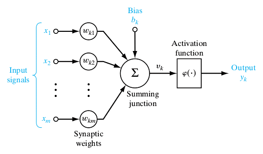
A single neuron is a computational unit with scalar inputs and outputs. There is a weight associated with each input to the neuron. The neuron multiplies each input by the associated weight and then sums up all the results. The result is then passed through a non-linear function whose result is the output of the neuron. Figure 1 shows a computation performed by a single neuron. The non-linear function is also known as the activation function of the neuron. The weights associated with the inputs are also known as synaptic weights in connection with the synapse in the human brain, over which electrical/chemical impulses pass from one neuron to another.
A number of neurons can be connected to each other, forming a neural network. The output of one neuron is connected as input to one or more other neurons forming a connected network. These connections can be organised in the form of layers, with outputs of neurons in one layer providing inputs to neurons in the next layer. The output of a neuron in one layer can be connected to one or all of the neurons in the next layer. The network in which each neuron’s output from one layer is connected to all other neurons in the next layer is known as a fully connected neural network. Neural networks typically contain one input layer, one output layer and one or more intermediate layers. The intermediate layers are also known as hidden layers.
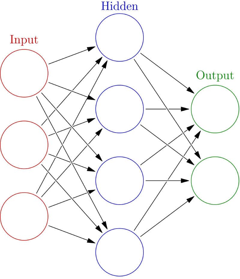
The simplest neural network is a network that contains one input layer, one intermediate layer/hidden layer and one output layer. An example of such a network is shown in Figure 2. Networks with two or more hidden layers are known as deep neural networks. A historical note on the evolution of neural networks can classify them as belonging to one of the three generations. This classification is based on the computational ability of the individual neuron used in the neural network.
The first generation of neural networks was based on neurons that were threshold gates or perceptrons. These neurons did not have a non-linear activation function; instead, their output was either 1 or 0, depending on whether the weighted sum of their inputs was above or below a threshold ‘t’. An important feature of these neural networks is that they can only produce digital outputs. However, they are capable of modelling every Boolean function and hence are universal for computation with digital inputs and outputs.
The second generation of neural networks consists of neurons which apply a non-linear continuous function to the sum of weighted inputs, and hence produce a continuous set of possible output values. Some of the examples of activation functions are the sigmoidal and tanh functions. A typical example of second generation neural networks is the feed forward neural network such as the one shown in Figure 2, which we discussed earlier. Other examples of second generation neural networks include recurrent neural networks and recursive neural networks, which we will discuss in subsequent columns.
Feed forward neural networks are those in which signals travel only in one direction, i.e., from input to output. In other words, the output of an earlier layer in the architecture feeds only to later layers and not the other way around. The output of any layer is not fed to itself or any other earlier layers in feed forward neural networks. The example shown in Figure 2 is a feed forward neural network. On the other hand, recurrent neural networks can have the output of one layer being fed back through the network into an earlier layer, over time.
Essentially, this means that the neural network has loops or cycles in which it allows the output computed at layer ‘i’ at time ‘t’ being fed back to an earlier layer at time ‘t+1’. This allows the recurrent neural networks to achieve some form of short-term memory. While feed forward neural networks are used for single input value classification, recurrent neural networks are typically used for sequence classification and time series classification.
Second generation neural networks can also support digital outputs by applying a threshold at the output, and hence can model any arbitrary Boolean function. They are also universal for analogue computations, since any continuous function can be approximated reasonably well by means of a second generation neural network with a single hidden layer itself.
Today, these second generation neural networks are widely used in various applications such as speech processing, image recognition and natural language processing. These neural networks are typically trained using gradient descent algorithms and back propagation. In order to apply neural networks to different tasks, one of the important challenges is how to effectively and quickly train these neural networks. In fact, one of the reasons for the resurgent popularity of artificial neural networks is that they can be trained efficiently using GPUs.
The third generation of neural networks employs spiking neurons, also known as ‘integrate and fire’ neurons. These neural networks more closely model the biological neurons’ activity compared to first and second generation neurons. These spiking neural networks can also be used for information processing, just as the second generation of neural networks. While their effectiveness has been described theoretically, they have not yet been widely used in real life applications due to their high computational demands. Hence, we will not discuss spiking neural networks, except to note that there is considerable research happening in this field. For instance, Qualcomm recently announced that Qualcomm Zeroth processors are based on the principle of spiking neural networks, which is an example of neuromorphic architectures—otherwise known as biologically inspired computing architectures.
We need to mainly focus on the second generation neural networks, since large real life natural language processing applications have been built using them.
The main application of neural networks in information processing is to use them as classifiers. In traditional machine learning (ML), different classifiers such as logistic regression classifiers and support vector machines are popularly used to classify text, images or speech. Similarly, fully connected neural networks can be used in place of traditional ML classifiers such as SVM, as a drop-in replacement for them. In many cases, neural network based classification has been shown to be more accurate than traditional ML learners. It is also important to note that extensive feature engineering, which has been associated with traditional ML learners, need not be done in the case of neural networks. Only core features are fed as input to the neural network and the network itself can learn additional features on its own.
While we have so far been talking about inputs to individual neurons in a neural network, we can, in fact, treat the inputs coming into each layer of a neural network as a vector, thus simplifying the mathematical calculations. The weights of the connections between the different layers will be represented using matrices. A fully connected layer is an implementation of a vector-matrix multiplication, where the incoming input vector X is multiplied by the weight matrix W of the connections.
If you have any favourite programming questions/software topics that you would like to discuss on this forum, please send them to me, along with your solutions and feedback, at sandyasm_AT_yahoo_DOT_com.


[…] to enable an integrated machine learning experience on Chrome browser. The library helps to train neural networks without requiring any app […]