


This article is intended to help developers who are working on machine learning initiatives or are planning to set out on this path. It is important to know about some basic concepts and steps when it comes to applying machine learning to real business problems.
Machine learning is a field of artificial intelligence (AI), in which systems are programmed to gather insights from historic data and generate outcomes that can be used for decision making. Machine learning problems can be approached in multiple ways, one of which is collecting lots of data and training the model. We can also derive features from the data and use them to train the model, or pre-process data and transform it into specific formats before using it to train a model. It is not easy to tell which approach will work and give the desired results. Hence, experts suggest some guidelines to approaching a machine learning problem:
- Start with a simple algorithm, then implement and test it with a small data set.
- Plot learning curves to see how it works, and if required, use more data or features.
- Perform error analysis to analyse errors and try to identify a pattern that can help in improving the algorithm.
It is not always recommended that you start with programming a machine learning algorithm but, instead, try it using open source tools such as R or Octave to play around and select the right model that works for particular types of data.
The objective of this article is to highlight some aspects that are important when selecting an algorithm, setting parameters and diagnosing performance. Some fundamental terms which are referred to in the article are explained below.
Hypothesis: A function that fits the data in linear or non-linear fashion
ŷ = hθ(x) = θ0+θ1x
Here, the hypothesis function is the equation line; so data will be fitted in a line. We give hθ(x) values for parameters θ0 and θ1 to get our estimated output ŷ.
Cost function: This is a function that is used to measure the accuracy of the hypothesis function, i.e., how well it fits the data. The function can be described as follows:
J(θ0,θ1) = (½m) ∑ (ŷ i−yi)2 = (½m) (hθ(xi)−yi)2 , for i=1 to m
To simplify this, it is where x is the mean of the squares of hθ(xi)−yi , or the difference between the predicted value and the actual value.
Gradient descent: This is a technique to estimate the parameters θ0 and θ1 of the hypothesis. The gradient descent equation for linear regression using a single variable is given below:
repeat until convergence: {
θ0 := θ0−α (1/m) ∑ (hθ(xi)−yi) , for i=1 to m
θ1 := θ1−α (1/m) ∑ ((hθ(xi)−yi) xi) , for i=1 to m
}
…where, m is the size of the training set and xi, yi are values of the given training set (data).
Regularisation: This keeps all the features but reduces the weightage.
minθ ½m [ ∑(hθ(x(i))−y(i))2+λ ∑(θj)2 ] , for i=1 to m and j=1 to n
λ, or lambda, is the regularisation parameter. It determines how much the cost of the θ parameters is inflated in order to reduce the weightage of the feature in the hypothesis function.
Evaluating a hypothesis
There is a misconception that the algorithm that produces low errors is also accurate. This may not always be the case, and the main reason for this could be overfitting. Overfitting (high variance) is caused by a hypothesis function that fits the available data well but does not generalise to predict new data. So it is very important to understand whether the algorithm is overfitting or underfitting (high bias), when the hypothesis function (h) maps poorly to the trend of the data. The following section provides some general guidelines to evaluate various aspects of the hypothesis/algorithm.
Model selection: Model selection is the process by which we choose the hypothesis with the least errors (more generalised), set parameters and identify any pre-processing requirement to predict the best results. However, it has been observed that errors will always be low on the data used for training the model compared to any other data. Hence, experts recommend another approach using a cross-validation set as detailed below.
- Split the dataset into three sets—a training set, a test set and a cross-validation set. The possible breakdown could be 60-20-20.
- Optimise the parameters in θ using the training set.
- Find the polynomial degree d with the least error using the cross-validation set.
- Estimate the generalisation error using the test set.
In this way, the degree of the polynomial (d) has not been trained using the test set and, hence, the generalisation error can be minimised.
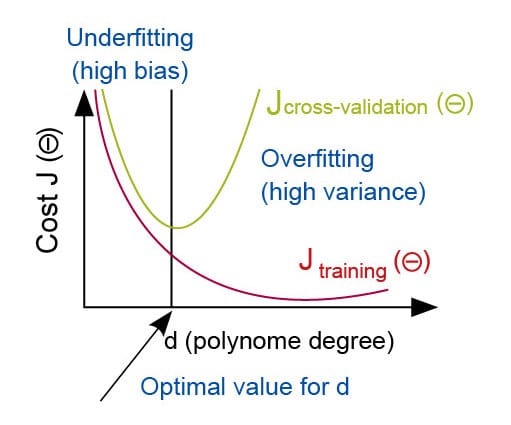
Diagnosis of bias vs variance: The study of relationships between the cost function and the degree of the polynomial (d) can help us determine whether underfitting or overfitting is the problem with our hypothesis. Here are some trends to look for during the diagnosis of bias and variance.
- Errors on training data decrease when we increase the degree of polynomial (d).
- Cross-validation errors decrease on increasing (d) up to a certain point, and then start to increase again.
Figure 1 summarises these trends.
Underfitting happens when (d) is small, and errors on both training data and cross-validation data are high. Overfitting happens when (d) is large, and training data errors are low while cross-validation errors are comparatively higher.
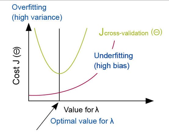
In case of regularisation, we can use the regularisation parameter λ to determine high bias/variance. The rule of thumb to use is:
- Large λ: High bias (underfitting)
- Intermediate λ: Just right
- Small λ: High variance (overfitting)
The relationship of λ to the training and cross-validation errors is shown in Figure 2.
Underfitting happens when λ is large, and errors on both training and cross-validation data are high.
Overfitting happens when λ is small, and errors on training data are low while cross-validation errors are high.
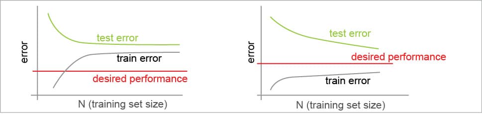
Learning curves: Learning curves can help in choosing the best value for (d) or λ to plot them. They can help us understand the relationship between errors and the test data size in situations of high bias/variance.
In case of a hypothesis with high bias (see the left of Figure 3):
- Low data size causes training errors to be low and cross-validation errors to be high.
- Large data size causes both training and cross-validation errors to be high (very similar) and become stable.
This means that the algorithm suffers from high bias. So getting more training data will not be very useful for further improvement.
In case of a hypothesis with high variance (see the right of Figure 3):
- Low data size causes training errors to be low and cross-validation errors to be high.
- Large data size causes training errors to increase and cross-validation errors to decrease (without stabilising).
This means that the algorithm suffers from high variance, so getting more training data may be useful.
Error metrics for skewed classes: The data sets is largely skewed when we have many more samples of one class compared to other classes in the entire data sets. In such a situation, we can use two attributes of the algorithm, called Precision and Recall, to evaluate it. In order to determine these attributes, we need to use the following truth table.
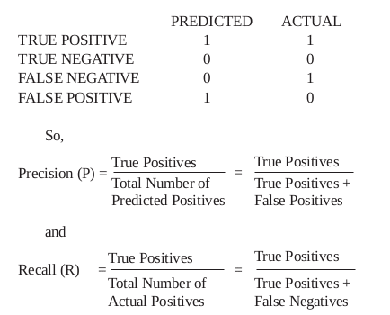
We need both Precision and Recall to be high for the algorithm to perform better. Instead of using these separately, there is a simpler solution—combining them in a single value called F1 score. The formula to calculate the F1 score is:
F1 Score = 2 (PR/P+R)
We need a high F1 score (so both P and R should be large). Also, the F1 score should be obtained over the cross-validation data set.
A few rules for running diagnostics are:
- More training examples fix high variance but not high bias.
- Fewer features fix high variance but not high bias.
- Additional features fix high bias but not high variance.
- The addition of polynomial and interaction features fixes high bias but not high variance.
- When using gradient descent, decreasing lambda can fix high bias and increasing lambda can fix high variance (lambda is the regularisation parameter).
- When using neural networks, small neural networks are more prone to underfitting and big neural networks are prone to overfitting. Cross-validation of the network size is a way to choose alternatives.
Tips on using the most common algorithms
SVM: SVM is one of the most powerful supervised algorithms. Listed below are some tips to applying the SVM algorithm:
- If the feature set (n) is large relative to the data sets size (m), then use SVM with logistic regression or linear kernel. We don’t have enough examples, which would have required a complicated polynomial hypothesis.
- If n is small and m is intermediate, then use SVM with a Gaussian Kernel. We have enough examples so we may need a complex non-linear hypothesis.
- If n is small and m is large, then manually create/add more features, and use logistic regression or SVM without a kernel. Increase the features so that logistic regression becomes applicable
K-Means: K-Means is most popular and a widely used clustering algorithm for unsupervised data sets. Some tips on applying K-Mean are listed below:
- Make sure the number of your clusters is less than the number of your training examples.
- Randomly pick K training examples (be sure the selected examples are unique). Determine K by plotting it against the cost function. The cost function should reduce as we increase the number of clusters, and then flatten out. Choose K at the point where the cost function starts to flatten out.
The availability of so many machine learning libraries today makes it possible to start building self-learning applications. However, when we talk about applying machine learning algorithms to real business problems, they need to be highly generalised, scalable and accurate in their outcome – be it prediction or clustering. This is not a very easy task, and requires a process involving various steps to make the algorithms work in the desired fashion.


