


A real-time, distributed search and analytics engine, ElasticSearch is used for full text search, structured search, analytics, and all three in combination. In short, it helps us to make sense of all the data thats being hurled at us every day.
Every year, billions of gigabytes of data are generated in various forms. We are swimming in an ocean of data. For many years, we have focused on generating and storing data in different structured forms. This data is not useful to us unless we can get some insights into it using analytics. We need tools to explore the data, and present it in a reader-friendly manner or in visual forms, so as to make sense out of it. It is rightly said that a picture is worth a thousand words.
There are many tools in the market for analytics, and ElasticSearch stands out among them. It is an open source tool with which we can analyse data. According to its website, ElasticSearch is a real-time, distributed search and analytics engine. It is used for full text search, structured search, analytics and all three in combination.
ElasticSearch is built on Apache Lucene, which is an open source library for high-performance, full-featured text search [https://lucene.apache.org/core/]. As Apache Lucene is a library, we need to do a lot of coding to integrate it with existing applications. The Apache Lucene library is built in Java; hence, the latter is required to use the former. ElasticSearch uses Apache Lucene internally for indexing and searching, but hides its complexities by providing access to the API in the form of the RESTful API, using JSON as the format for exchanging data.
ElasticSearch is a product of the Elastic Company, which was founded in 2012. The firm has also built Logstash, Kibana and Beats, all of which are open source projects. Apart from these, there are some commercial products available like Marvel, Shield, Watcher, Found, etc. More details about the products and what they do can be found at https://www.elastic.co/products.
For this article, we will use ElasticSearch to store, search and analyse the data. We will also use Kibana to visualise and explore the data. The remaining products are out of the scope of this article.
Well-known users of ElasticSearch
Facebook, Microsoft, NetFlix, Wikipedia, Adobe, Stackoverflow, eBay and many other companies are using ElasticSearch in various ways to explore and analyse data. More details in the form of use cases are available online at https://www.elastic.co/use-cases.
Installation and configuration
ElasticSearch needs a recent version of Oracle JVM, i.e., JDK 1.7U55, or higher. For more details, refer to https://www.elastic.co/support/matrix#show_jvm.
ElasticSearch can be downloaded from https://www.elastic.co/downloads/elasticsearch. It comes in a variety of formatsZip, tar, DEB and RPM. DEB and RPM are packages for Linux based systems. We will go with the Zip format. Download the Zip file and extract it.
In the extracted folder, locate the config folder and open elasticsearch.yml in editing mode. In Linux based systems, simply right click and open the file using Gedit or a similar editor. On Windows, use Notepad or some other text editor.
In the elasticsearch.yml file, let us set some basic information:
- Find the line cluster.name: my-application. Remove the # sign so as to uncomment the line. Replace my-application with some other more meaningful name.
- Find the line node.name: node-1, uncomment it by removing # at the start of the line and replace node-1 with some meaningful name.
- Find the network.host: 192.168.0.1, uncomment it and instead of the IP address, specify 127.0.0.1.
- Save and close the file.
To run ElasticSearch, open the command prompt or terminal, and navigate to the bin directory. For Windows, it has batch files, and for Linux it has sh files.
- On a Windows system, execute elasticsearch.bat on the command prompt.
- On a Linux system, execute ./elasticsearch in a terminal.
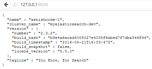
- Open the browser address 127.0.0.1:9200, as shown in Figure 1.
It shows that ElasticSearch is working. We can see the node name and the cluster name that we specified in elasticsearch.yml file.
This can also be tested using the curl command, which is available on Linux systems by default. For Windows, download curl.exe and add the same to the path. We dont require it for this article its been mentioned just for better understanding.
Open the terminal and run the following commands, one by one:
curl http://127.0.0.1:9200/
curl http://127.0.0.1:9200/?pretty
Using curl is not very comfortable, especially for beginners. We need a tool to visually interact with the ElasticSearch RESTful APIs. At the end, we would like to visualise the data also.
To do so in ElasticSearch, Kibana is used along with Sense, which is a Kibana plugin that allows a visual interaction with the RESTful API of ElasticSearch.
Download Kibana from https://www.elastic.co/downloads/Kibana. Download the appropriate versions of Windows or Linux. Extract the downloaded Zip file.
Open the command prompt or terminal and navigate to the Kibana folder. On a Linux machine, execute the following command:
./bin/Kibana --install elastic/sense
On a Windows machine, navigate to the bin folder inside the extracted Kibana folder and execute the following command:
kibana.bat plugin --install elastic/sense
This will install the Sense plugin from the Web.
We need to start Kibana by running kibana.bat on Windows and ./kibana on a Linux machine both files can be found in the bin directory.
In a browser, open a new tab and in the address bar, type http://127.0.0.1:5601 and press Enter. This will display the Kibana dashboard. We can configure it in a later section [i.e., visualising the data].
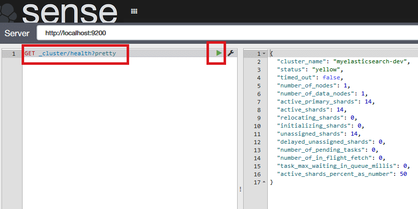
Modify the URL to http://127.0.0.1:5601/app/sense. It will display a two-pane window. The left pane is used to format the request for ElasticSearch and the right pane will display the response to the request. In the left pane, type GET _cluster/health?pretty and press the small green arrow button as shown in Figure 2.
While you are typing, Sense will provide auto completion for APIs. This can also be achieved using curl but the Sense plugin is a better option.
In the next section, we will use Sense to store, search and analyse data.
Storing, searching and analysing data
Storing data: Let us assume that we want data about students to be analysed. We will store the data, using the ElasticSearch RESTful API. We will create a student with the following attributes first name, gender, city, state, SSC, HSC, graduate degree, goal and hobbies. The attributes SSC, HSC and graduate degree will store percentage as value.
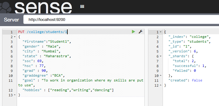
We need to use the PUT request to store [ create / update ] the data. Use the following command in Sense [Figure 3]:
PUT /college/students/1
{
firstname:Student1,
gender : Male,
city : Mumbai,
state : Maharastra,
ssc: 69,
hsc : 77,
grad : 90,
graddegree :BCA,
goal : To work in organization where my skills are put to use,
hobbies : [reading,writing,dancing]
}
The act of storing the data in ElasticSearch is called indexing. The diagram shows a student document. For every student, a document will be made. This data is stored in clusters, which can contain many indices.
So each student is a document or rather, we can say that the document is of type student. It is stored in the college index, which in turn is stored in a cluster. When we say /college/student/1 it is interpreted as /index/type/id. This is clear from Figure 3, which displays _type, _index, _id as a response to the request.
Similarly, lets create some more students so that we can analyse the documents. While adding data, make sure to have variations in gender, state, city, hobbies and goals.
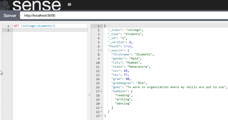
Querying data: To query or search the data stored, the ElasticSearch API uses the GET method followed by the URL. For example, to retrieve the record of Student 1, execute the following command, which is shown in Figure 4.
GET /college/students/1
To search the data, use GET /college/students/_search, which will return all students records.
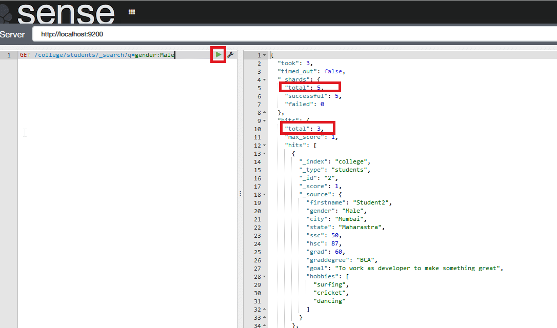
To search for data, where the gender is male, use: GET college/students/_search?q=gender:Male
and it will return all male students as shown in Figure 5.
In the results, we can see that of a total of five student documents, three are of males.
Similarly, we can search the data using other fields. But this syntax will be difficult for and/or criteria. ElasticSearch provides query DSL or the Domain Specific Language to get the data. Learning DSL will take some time. The following sections show how to write queries using DSL. For example, to search all male students who also have the hobby of reading, use the commands given below:
GET /college/students/_search
{
"query":{
"bool": {
"must" :{"match":{"hobbies": "reading"}},
"must" :{"match":{"gender":"Male"}}
}
}
}
Lets search the goal field to find what contains the text works as, as follows:
GET /college/students/_search
{
"query":{
"match" : {
"goal" : "work as"
}
}
}
This will display all the students whose goal contains the words works as or work.
We have covered how to store and search for data using ElasticSearch. Now, the last part is to analyse the data.
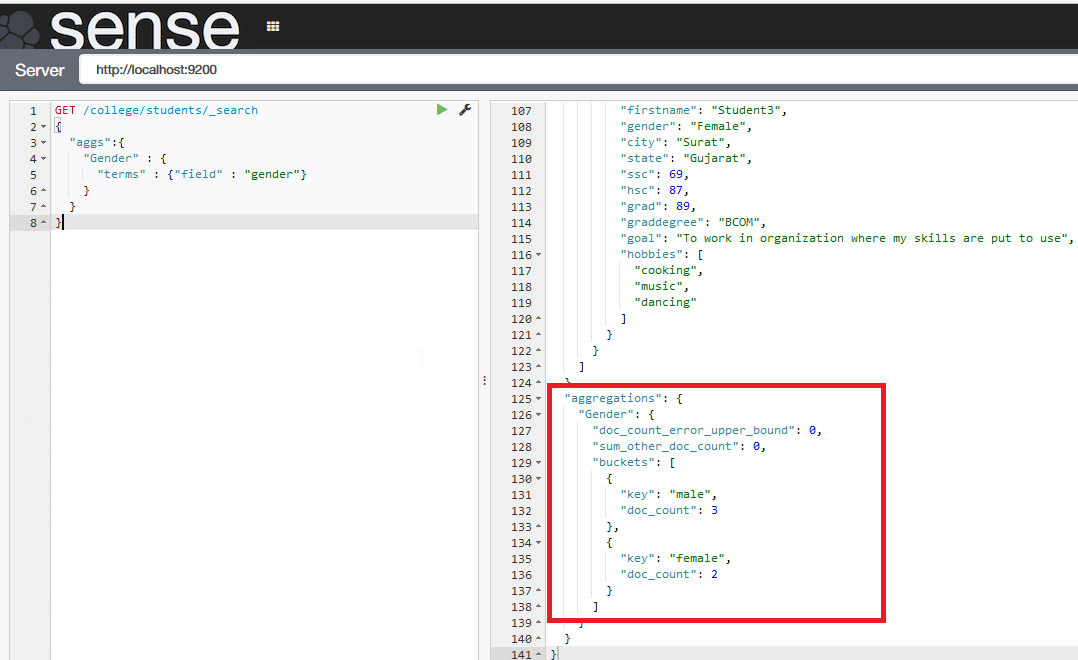
Analysing data: To analyse the data, aggregators are provided something like group by in SQL. For example, if we need to find the number of male and female students, refer to Figure 6.
GET /college/students/_search
{
"aggs":{
"Gender" : {
"terms" : {"field" : "gender"}
}
}
}
There are many other ways to think of for aggregators. For more details, you could refer to online documentation.
Visualising data
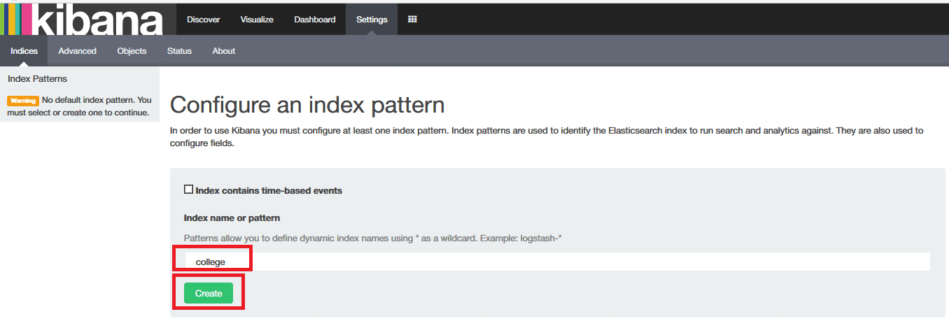
In the previous section, we used ElasticSearch to store, search and analyse the data. But the actual power comes with the visualisation of data. Assuming your ElasticSearch and Kibana are up, open a browser, enter the URL 127.0.0.1:5601 and press Enter. In the text box, enter College as we are going to use our college index for visualisation. Then click on the Create button as shown in Figure 7.
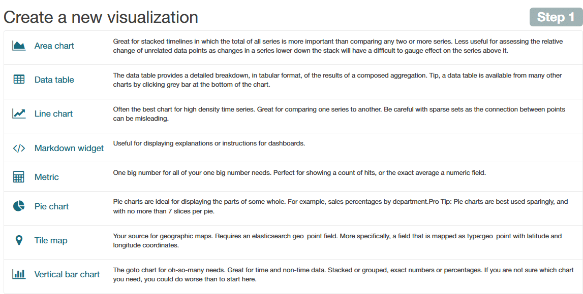
On the top bar, click on Visualisation, which will show various options for creating new visualisation, as shown in Figure 8.
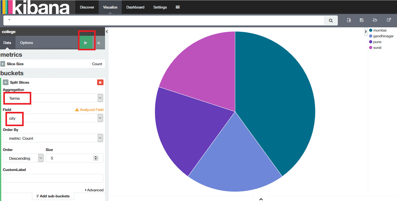
Select Pie Chart, and it will ask you to Select Search Source. Choose From a New Search. It will display a pie chart and some options to use on the left side. Locate Buckets, which will show the option Split Slices. Click on Split Slices, then onSelect Terms in Aggregation, and in Field select State before clicking on the white arrow button within a green square, as shown in Figure 9.
We can see that this has created the pie chart for the city, where the slices are based on the number of students from each city. On the right side, we can see different cities and the colours they represent.
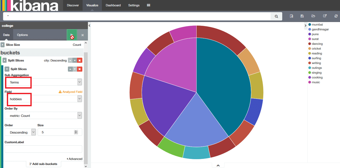
Lets add more to this pie chart. On the left side bottom there is the option to Add Sub buckets. Click on it. Repeat the procedure, i.e., click on Split Slice, and then on Select Terms in Sub Aggregation. Then select Hobbies in Fields, and click on the white arrow button. You will get whats shown in Figure 10.
Once done, we can save this visualisation for future use, so that the next time we dont have to configure all parameters.
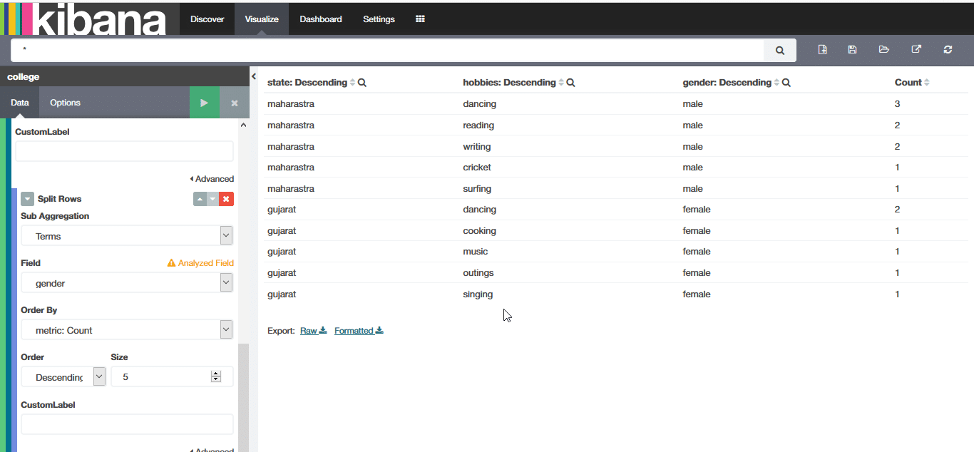
Let us think of other examples, for instance, if we want to know statewise hobbies of students on a gender basis. We can create a data table from the visualisation and can get something like Figure 11.
Once you have data, the possibilities are endless regarding what you can extract from it. The data has all the answers. We only need to ask the right questions.


Thanks ! Well explained