


In the past two issues, we have dealt with many tools necessary to learn ns-3, which is a system of software libraries that work together to form a wonderful simulation tool. There are a lot of system libraries that are part of ns-3, and the user programs are written so that they can be linked to the core library. Let us first discuss the different classes available with ns-3 and the way they imitate and act as an abstraction of real world network entities. It may not always be feasible or possible to imitate a real world entity completely, with computer simulation. In such situations, we need to scale down things a bit, so that computers can handle the complex and confusing real world entities, without losing the essential characteristics of the particular entity being simulated. So an abstraction is a simplified version of an entity, with its essential characteristics. In order to set up a network, we need computer systems (nodes), applications running on top of these nodes, network devices for connectivity and connecting media. The section below discusses these real world entities and a few ns-3 abstracting classes imitating them.
A few built-in classes in ns-3
Node: In computer networking, node represents a host computer. In ns-3, the term node has a slightly different meaning. A C++ class, called Node, is used to implement nodes in ns-3 simulation. A node is a simplified model of a computing device in ns-3 and by creating an object of the Node class, you are actually creating a computing device in the simulation. For example, if there are 10 objects of the Node class in your simulation script, then you are simulating a network with 10 nodes. This is the power of ns-3. The developers of ns-3 have already finished the code required in your scripts to imitate a node in the real world; all you need to do now is call the Node class to create an object that imitates a real node.
Application: The behaviour of the application programs running on a real computer in a network is imitated by the Application class of ns-3. Using this class, a simple application can be installed on top of a node. A real computer node can have complex software like operating systems, system software and applications, but in ns-3, we content ourselves with simple applications, which are in no way comparable to real world software. Examples of applications are BulkSendApplication, OnOffApplication, etc. The BulkSendApplication is a simple traffic generator which will send data as fast as possible up to a maximum limit or until the application is stopped. The OnOffApplication is also a traffic generator and it follows an On/Off pattern for sending data. During the On stage, this application maintains a constant bit rate data transfer and during the Off stage, no data is transferred.
The NetDevice class: In order to connect a computer to a network, certain network devices like network interface cards, cables, etc, are required. Even while simulating a network of computers, we cannot ignore network devices and ns-3 has a class named NetDevice for this purpose. The NetDevice class in ns-3 provides an abstraction which, if used with the Node class, will imitate a real world computer with a network device installed on it. Just like an application, a network device in ns-3 is also a simplified abstraction, which in no way resembles a complex real world network device. In fact, the NetDevice abstraction class in ns-3 acts as a device driver as well as simulated hardware. There are several specialised variants of the NetDevice class called CsmaNetDevice, PointToPointNetDevice, WifiNetDevice, etc.
Channels: In a real network, nodes are interconnected through a medium or a channel. For example, we can connect two nodes with a twisted pair cable or a wireless channel. There is a class called Channel in ns-3 which acts as an abstraction of a real world channel. The Channel class acts as a basic framework for all the other specialised channel classes in ns-3. There are specialised channel classes like CsmaChannel, PointToPointChannel, WifiChannel, etc.
Our first ns-3 script
Now that we have discussed ns-3 classes imitating real world entities, it is time to deal with our first ns-3 script. The simulation script given below contains only absolutely essential code for simulating a very simple network in the real world. The simulated network contains just two nodes with a point-to-point connection between them. This is a slightly modified version of a program taken from the standard set of examples bundled with ns-3. I have removed some lines of code from the original program, which might distract from the core issues related to ns-3 simulation.
#include ns3/core-module.h
#include ns3/network-module.h
#include ns3/internet-module.h
#include ns3/point-to-point-module.h
#include ns3/applications-module.h
using namespace ns3;
NS_LOG_COMPONENT_DEFINE(SimulationOne);
int main(int argc, char *argv[ ])
{
Time::SetResolution(Time::NS);
LogComponentEnable(UdpEchoClientApplication, LOG_LEVEL_INFO);
LogComponentEnable(UdpEchoServerApplication, LOG_LEVEL_INFO);
NodeContainer nodes;
nodes.Create(2);
PointToPointHelper pointToPoint;
pointToPoint.SetDeviceAttribute(DataRate, StringValue (10Mbps));
pointToPoint.SetChannelAttribute(Delay, StringValue (5ms));
NetDeviceContainer devices;
devices = pointToPoint.Install(nodes);
InternetStackHelper stack;
stack.Install(nodes);
Ipv4AddressHelper address;
address.SetBase(192.168.100.0, 255.255.255.128);
Ipv4InterfaceContainer interfaces = address.Assign(devices);
UdpEchoServerHelper echoServer(2000);
ApplicationContainer serverApps = echoServer.Install(nodes.Get(1));
serverApps.Start(Seconds(1.0));
serverApps.Stop(Seconds(10.0));
UdpEchoClientHelper echoClient(interfaces.GetAddress(1), 2000);
echoClient.SetAttribute(MaxPackets, UintegerValue(2));
echoClient.SetAttribute(Interval, TimeValue(Seconds(3.0)));
echoClient.SetAttribute(PacketSize, UintegerValue(512));
ApplicationContainer clientApps = echoClient.Install(nodes.Get(0));
clientApps.Start(Seconds(3.0));
clientApps.Stop(Seconds(12.0));
AsciiTraceHelper ascii;
pointToPoint.EnableAsciiAll(ascii.CreateFileStream(simulation1.tr));
Simulator::Run();
Simulator::Destroy();
return 0;
}
Before explaining the program, heres a word about the indent style used in ns-3 source files. ns-3 uses an indent style called the GNU style. It will be better if you follow this style with your ns-3 script files also. If you are unfamiliar with the GNU style of indenting, you could use a tool called Artistic Style which will format the program text in any style you prefer. Finally, a word of caution to die-hard fans of Vi and Vim; ns-3 prefers Emacs over Vi. Most often, ns-3 source files start with an Emacs mode line specifying the formatting style. Now let us break the script into small pieces and analyse it.
A few explanations
Even though the syntax of the program resembles C++, it is ns-3. I will explain only terms specific to ns-3 in the above example by making an assumption that the C++ constructs in the script are already known to the reader.
The script starts with five include statements. But these are not the only header files included in your script. These five header files will, in turn, include a large number of header files required for the proper working of the ns-3 simulation script. This may not be an optimal solution to our problem of including the required header files alone. But this approach definitely reduces the burden on the ns-3 script writer; instead, the burden is passed on to the system running the simulation with many unnecessary header files included. The next line using namespace ns3; makes every class, function and variable declared inside the ns-3 namespace available for direct usage without using the qualifier ns3::. Remember, we havent used the standard namespace std of C++. So we need the qualifier std:: to get standard C++ constructs, e.g., std::cout<< Hello ns-3; will work but cout<<Hello ns-3; will result in an error.
The next line NS_LOG_COMPONENT_DEFINE(SimulationOne); declares a logging component named SimulationOne. By referring to this logging object console, message logging can be enabled and disabled. Logging is one of the three methods used in ns-3 to provide simulation data to the user. The other two methods are trace analysis and network topology animation. Even though logging is a very useful way to obtain data from the simulation, the preferred method is trace analysis. With logging, the data is displayed on the terminal. There are seven different log types used in logging. These are: LOG_ERROR, LOG_WARN, LOG_DEBUG, LOG_INFO, LOG_FUNCTION, LOG_LOGIC and LOG_ALL. The amount of information provided increases with each level, with LOG_ERROR providing the least information and LOG_ALL providing the most.
The next line Time::SetResolution(Time::NS); sets the least amount of time by which two events can be separated. The default minimum time is one nanosecond. Now consider the following two lines of code.
LogComponentEnable(UdpEchoClientApplication, LOG_LEVEL_INFO); LogComponentEnable(UdpEchoServerApplication, LOG_LEVEL_INFO);
For each log type there is a corresponding log level type, which enables logging of all the levels below it in addition to its level. So the above lines enable logging on the UDP echo client and UDP echo server with log level type LOG_LEVEL_INFO, which will display information from the log types LOG_ERROR, LOG_WARN, LOG_DEBUG and LOG_INFO. If you find this line confusing, dont worry. This line does not affect the topology of the network we are simulating; it only restricts the amount of data given to the user from the terminal. So, if you want, you can use LOG_LEVEL_ALL, which will provide you with all the available information, even that which is unnecessary for your analysis.
From the following line of code onwards, we are dealing with the actual network being simulated. Earlier, we discussed the different abstract network entities used in ns-3 simulation. All these entities are created and maintained with the help of corresponding topology helper classes.
NodeContainer nodes; nodes.Create(2);
The class NodeContainer in the above code is a topology helper. It helps us deal with the Node objects, which are created to simulate real nodes. Here we are creating two nodes by using the Create function of the object called nodes.
In the following lines of code, a topology helper class called PointToPontHelper is called to configure the channel and the network device:
PointToPointHelper pointToPoint; pointToPoint.SetDeviceAttribute(DataRate, StringValue (10Mbps)); pointToPoint.SetChannelAttribute(Delay, StringValue (5ms));
You can observe that the data rate of the network device is set as 10Mbps and the transmission delay of the channel is set as 5ms. If you are unfamiliar with network simulation altogether, then this is how things are done in a simulation. You can specify different values in a simulated network without making any marginal changes. For example, you can change the delay to 1ms or 1000ms. Thus, you can create fundamentally different networks by changing a few lines of code here and there. And that is the beauty of simulation.
The two lines of code shown below will finish configuring the network and the channel. Here, a topology helper called NetDeviceContainer is used to create NetDevice objects. This is similar to a NodeContainer handling Node objects.
NetDeviceContainer devices; devices = pointToPoint.Install(nodes);
So now, we have nodes and devices configured. Next, we should install protocol stacks on the nodes. The lines InternetStackHelper stack; and stack.Install(nodes); will install the Internet stack on the two nodes. Internet stack will enable protocols like TCP, UDP, IP, etc, on the two nodes.
The next three lines of code shown below deal with node addressing. Each node is given a specific IP address. Those familiar with ns-2 should note the difference. In ns-3, abstract IP addresses used in the simulation are similar to actual IP addresses.
Ipv4AddressHelper address; address.SetBase(192.168.100.0, 255.255.255.128); Ipv4InterfaceContainer interfaces = address.Assign(devices);
The subnet mask is 255.255.255.128; therefore, the possible IP addresses are from 192.168.100.1 to 192.168.100.126. Since there are just two nodes, the addresses are 192.168.100.1 and 192.168.100.2.
During our discussion on ns-3 abstractions, I mentioned abstract applications running on ns-3 nodes. Now it is time for us to set up abstract applications on top of the two nodes. The lines from UdpEchoServerHelper echoServer(2000); to clientApps.Stop(Seconds(12.0)); in the script simulation1.cc are used to create abstract applications on the two nodes. The node with address 192.168.100.1 is designated as the client, and the node with address 192.168.100.2 is designated as the server.
Initially, we create an echo server application on the server node. The port used by the echo server is 2000. The line ApplicationContainer serverApps = echoServer.Install(nodes.Get(1)); installs a UDP echo server application on the node with ID 1. The server application starts at the first second and stops at the tenth second. Then we create a UDP echo client on the node with ID 0, and it connects to the server with the line UdpEchoClientHelper echoClient(interfaces.GetAddress(1), 2000);. Remember the connection mechanisms we learned in socket programming? With the next three lines of code, the maximum number of packets sent is set as two, the interval is set as 3 seconds and the packet size is fixed as 512 bytes. The client application starts at the third second and stops at the twelfth second. So with the simulation script given above we have created nodes, installed applications on the nodes, attached network devices on the nodes, and connected the nodes to a communication channel. Thus our topology is complete and we are ready to begin the simulation. And finally, the lines Simulator::Run(); and Simulator::Destroy(); start and stop the actual ns-3 simulator.
Trace files in ns-3
I have explained every line of code in the script simulation1.cc except the following two lines:
AsciiTraceHelper ascii; pointToPoint.EnableAsciiAll(ascii. CreateFileStream(simulation1.tr));
These two lines are included in the script for trace file generation. Trace file analysis is the main source of information in ns-3 simulation. There are two different types of trace files in ns-3. They are ASCII based trace files and pcap based trace files. pcap is an application programming interface (API) for capturing network traffic. A packet analyser tool called Wireshark is used to process the pcap files to elicit information. Initially, we will only discuss the relatively simple ASCII based tracing method. The code given above will generate an ASCII trace file named simulation1.tr. The text below shows only the first line of the trace file.
+ 3 /NodeList/0/DeviceList/0/$ns3::PointToPointNetDevice/TxQueue/Enqueue ns3::PppHeader (Point-to-Point Protocol: IP (0x0021)) ns3::Ipv4Header (tos 0x0 DSCP Default ECN Not-ECT ttl 64 id 0 protocol 17 offset (bytes) 0 flags [none] length: 540 192.168.100.1 > 192.168.100.2) ns3::UdpHeader (length: 520 49153 > 2000) Payload (size=512)
You can download the simulation script simulation1.cc and the corresponding trace file simulation1.tr from opensourceforu.com/article_source_code/july2015/ns3.zip. The ASCII trace files in ns-3 are similar in structure to ns-2 trace files. There is abundant data available in the form of a trace file in ns-3. A detailed description of the different fields in the trace file and ways to elicit information from this file will be discussed in the next issue.
Executing the script
Now that we are familiar with the code, lets move on to the execution of the code. If you have installed ns-3 inside a directory called ns as discussed in the last article of this series, you will have the following directory ns/ns-allinone-3.22/ns-3.22/scratch. Copy the file simulation1.cc into the directory called scratch. You have to copy ns-3 scripts into this directory so that the build automation tool, Waf, can identify and compile them. Now open a terminal in the directory ns/ns-allinone-3.22 and type the following command:
./waf
If your script is incorrect, you will see error messages displayed on the terminal. If the simulation script is correct, you will see a message regarding a list of modules built and a few modules not built. If you see such a message, then type the following command in the terminal:
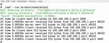
./waf - - run scratch/simulation1
This command will execute the simulation script simulation1.cc. Figure 1 shows the terminal with logged information displayed. From the figure, we can see that the client sends 512 bytes of data to the server at the third second. The server responds with 512 bytes of data to the client. After a waiting period of 3 seconds, at the sixth second, the client again sends 512 bytes to the server and the server in turn responds by sending 512 bytes of data to the client.
Graphical animation in ns-3
We have briefly discussed the NAM graphical animator used with ns-2 in the first part of this series. We are now going to deal with network animation in ns-3. Unlike ns-2, there is no single default animator for ns-3. But we have two tools called NetAnim and PyViz for network animation in ns-3. PyViz is a live simulation visualiser, which means it doesnt use trace files. NetAnim is a trace based network animator. I will stick to NetAnim, because those who are familiar with ns-2 will find NetAnim similar to NAM. NetAnim is an offline animator based on the Qt toolkit, and uses XML based trace files generated by ns-3 scripts to display the animation. The latest version is NetAnim 3.106. But the version bundled with the ns-3.22 tarball installation file is NetAnim 3.105. If you have installed ns-3 inside a directory called ns, then you will have the directory ns/ns-allinone-3.22/netanim-3.105. Open a terminal in this directory and type the following command:
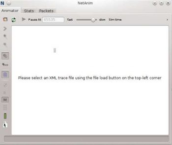
./NetAnim
Figure 2 shows the NetAnim window you are supposed to see. But theres an error message because the executable file called NetAnim is not there. What has happened is that with the tarball installation of ns-3, NetAnim did not get installed. So we need to install NetAnim separately. But thats for another day. So in the next part of this series, we will learn how to install and use NetAnim. Thereafter, we will also deal with ns-3 trace files in detail.


Very informative and helpful for new learners.