


Scilab (http://www.scilab.org) is open source software for numerical computation with a syntax similar to MathWorks MATLAB. The first part of this article is about the use of LaTeX with Scilab, and the second concerns the keywords and how to use them to build a syntax highlighting file for GNU Emacs and Vim. All the code presented here has been tested with Scilab 5.5.1 under Linux Mint 17 Xfce. Since the full code is too long for a printed article, its freely (as in freedom and in beer) available at https://github.com/astonfe/scilab
LaTeX on a plot
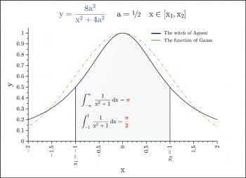
Version 5.2 is the first version of Scilab in which it is possible to use LaTeX. The rendering engine is based on JLaTeXMath (see Reference 1), a fork of JMathTeX (Reference 2) which is a Java library for the mathematical mode of LaTeX. Its not necessary to install LaTeX to use it with Scilab. Lets consider the plot shown in Figure 1, which shows two bell-shaped curves: the witch of Agnesi (Reference 3) and the function of Gauss. This plot has seven textual parts:
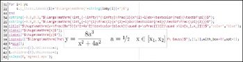
1. Title. The syntax is: title($this-is-the-title$,color,color-name). First, its necessary to consider that a text written in LaTeX must be included between two $ symbols. In this example, the full title is written in the colour blue. Two or more colours are possible by adding the LaTeX command \textcolor. On the plot, I can see the first part written in blue and the second in black. If I put the mouse on the LaTeX code, SciNotes, the built-in editor shows, an all-black preview (Figure 2), while the blue part is not visible.
2. X axis label. The syntax is very easy: xlabel($this-is-the-label$).
3. Y axis label. The syntax with ylabel is the same as in the X axis.
4. X ticks labels. In this example, labels are defined as strings in the vector labx. Using x_ticks.labels within a loop, I can put each label on the plot. The syntax is: x_ticks.labels=$some-latex-here+labx+$.
5. Y ticks labels. In this example, they are numbers in a range between 0 and 1. The syntax is: y_ticks.labels=$some-latex-here+string(laby)+$ If laby=string(0:0.1:1), the syntax is the same as in the X axis.
6. Legend. This syntax is a bit long: legends([$first-row-text$;$second-row-text$],[first-row-color-number,second-row-color-number],with_box=%f,opt=1). The option with_box can be %f (false) or %t (true) and opt is an integer in the range from 1 to 6.
7. Two integrals under the curves. Another example of an easy syntax: xstring(x-position,y-position,$some-latex-here$). The area under the witch of Agnesi is equal to p, or p/2 under the grey part. In general, the area between the curve and the X axis is equal to 4 a2 p (in the example shown, a=1/2).
The full code for this example agnesi.sce is available on GitHub.
From Scilab to LaTeX
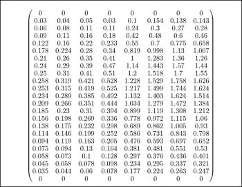
In the May 2015 issue of OSFY, on page 103, there is a ribbon plot that shows one absorbance spectrum measured at eight different times. The data matrix is composed of eight columns and 23 rows. I can export this matrix directly to LaTeX using the function prettyprint. For the first four rows, the result is shown in the following code (the remaining rows are replaced by the dots):
${\begin{pmatrix}0&0&0&0&0&0&0&0\cr 0.03&0.04&0.05&0.03&0.1&0.154&0.138&0.143\cr
0.06&0.08&0.11&0.11&0.24&0.3&0.27&0.28\cr 0.09&0.11&0.16&0.18&0.42&0.48&0.
6&0.46\cr ... \end{pmatrix}}$
Another way is to print the matrix in a graphic window with xstring(0,0,prettyprint(data)), as shown in Figure 3.
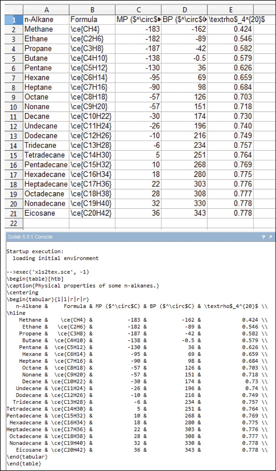
Its also possible to use Scilab as an almost automatic converter of tables from xls (via LibreOffice Calc) to LaTeX. The following code is composed of four parts: read the data from an xls table (text and numbers), get the maximum width of each column, print the column headers, and then print the data values. The caption and the tabular alignments are the only code rows that must be settled by hand. The original xls table is shown in Figure 4 (top); the output on Scilab Console is a table in LaTeX code that is fully formatted, as shown in Figure 4 (bottom). The data has been taken from Reference 4.
clear;
sheets=readxls(uigetfile(*.xls));
data=sheets(1);
typeof(data);
data.text;
data.value;
data=string(data);
[nr,nc]=size(data);
// Max width of each column
w=zeros(nc,1);
for i=1:nc
w(i)=max(length(data(:,i)));
end
printf(msprintf(\\\\begin{table}[htb])+\n..
+msprintf(\\\\caption{Physical properties of some n-alkanes.})+\n..
+msprintf(\\\\centering)+\n..
+msprintf(\\\\begin{tabular}{l|l|r|r|r})+\n);
// Columns headers
for i=1:nc
printf(%+string(w(i))+s,data(1,i));
if i<nc then printf( & );
end
end
printf( \\\\+\n+\\hline+\n);
// Data values
for i=2:nr
for j=1:nc
printf(%+string(w(j))+s,data(i,j));
if j<nc then printf( & );
end
end
printf( \\\\+\n);
end
printf(+msprintf(\\\\end{tabular})+\n..
+msprintf(\\\\end{table})+\n);
Keywords
The keywords of Scilab fall into five categories: primitives, commands, variables, functions and xcos functions. In my Scilab installation, five toolboxes GUI Builder, IPT3, JSON, NaN and Quapro are present, apart from some other dependencies that got automatically installed. The function getscilabkeywords returns a list with all the Scilab keywords already categorised.
clear; list_all=getscilabkeywords(); write(1_primitives.txt,list_all(1)); write(2_commands.txt,list_all(2)); write(3_variables.txt,list_all(3)); write(4_functions.txt,list_all(4)); write(5_xcosfuns.txt,list_all(5));
Now I have five text files. But there is a small problem. Some keywords are present in more than one file – the keywords extraction is not really perfect, so some deletions are necessary. The following keywords are removed from the functions file:
// Also present in primitives
datatipManagerMode
datatipMove
datatipSetOrientation
datatipSetStyle
// Also present in commands
apropos
help
// Also present in xcosfuns
lincos
scicos_simulate
steadycos
block_parameter_error
find_scicos_version
fixedpointgcd
get_scicos_version
initial_scicos_tables
returntoscilab
scicos_getvalue
scicos_workspace_init
with_modelica_compiler
Finally, I have five text files without any overlap: primitives with 1193 keywords, commands with 29 keywords, variables with 94 keywords, functions with 2462 keywords and xcosfuns with 12 keywords. The total is equal to 3790 keywords.
GNU Emacs
The keywords in each text file are sorted first by length and then alphabetically. Then its necessary to add the quotes before and after each keyword, merge every four lines (to reduce the number of rows) and add some Emacs Lisp code. A short example is given by the commands:
(setq scilab-commands ( endfunction continue function apropos elseif resume return select abort break catch clear pause while case else exit help quit then what clc end for pwd try who do if ))
Each keyword category is then submitted to GNU Emacs in the following order: scilab-xcosfuns, scilab-functions, scilab-primitives, scilab-commands, scilab-variables. Some modifications to the syntax table are also necessary to specify the comments highlighting and that some characters can be a keyword or a part of a keyword:
(modify-syntax-entry ?\/ . 12b synTable) (modify-syntax-entry ?\n > b synTable) (modify-syntax-entry ?_ w synTable) (modify-syntax-entry ?! w synTable)
As a result, I have the Scilab code highlighted with the default colours: five colours for the keywords, one colour for the strings and one colour for the comments. The default colours are quite different from each other, so further improvements are not necessary. Now all the keywords are recognised without any error. Last, add (require scilab-mode) to your dotemacs file. This syntax highlighting file for GNU Emacs has been made following the notes written by Xah Lee (see Reference 5). The full scilab-mode.el code is available on GitHub.
Vim
In the case of Vim, the keywords in each file are sorted only alphabetically, which is not necessary. I can also leave the keywords in the order in which they were originally extracted. Then merge every four lines (to reduce the number of rows) and add some Vim script code. Even in this case, a short example is given by the commands:
syn keyword sciCommands abort apropos break case
syn keyword sciCommands catch clc clear continue
syn keyword sciCommands do else elseif end
syn keyword sciCommands endfunction exit for function
syn keyword sciCommands help if pause pwd
syn keyword sciCommands quit resume return select
syn keyword sciCommands then try what while
syn keyword sciCommands who
Now its necessary to specify that some characters can be a keyword or a part of a keyword:
setlocal iskeyword+=!-!
setlocal iskeyword+=$-$
setlocal iskeyword+=%-%
Last, some Vim script code about the colours is added. As a result, I have the Scilab code highlighted with seven custom colours:
hi Operator guifg=#0000CD Medium blue hi Conditional guifg=#DC143C Crimson hi Statement guifg=#FF8C00 Dark orange hi Function guifg=#1E90FF Dodger blue hi Label guifg=#D2B48C Tan hi String guifg=#808080 Gray hi Comment guifg=#3CB371 Medium sea green HiLink sciPrimitives Operator HiLink sciCommands Conditional HiLink sciVariables Statement HiLink sciFunctions Function HiLink sciXcosfuns Label
My syntax highlighting file for Vim is partially based on those written by Vaclav Mocek (see Reference 6) and Patricio Toledo (Reference 7). The full scilab.vim code is available on GitHub.
Scilab has some interesting LaTeX capabilities about plots and data management. A syntax highlighting file is fairly easy to build for GNU Emacs and Vim. Its easy also for jEdit (Java based and cross-platform) and Notepad++ (Windows only). The interaction between Scilab and GNU Emacs, in a manner similar to ESS for R, is possible but does not really interest me, so I havent explored it yet. This article is the last of a series of four articles about Scilab, but I do think that, Scilab is a rare gem that is waiting to be discovered more broadly, as stated by Raphaël Auphan, the CEO of Scilab (see Reference 8).
References
[1] http://forge.scilab.org/index.php/p/jlatexmath, last visited on 25/04/2015.
[2] http://jmathtex.sourceforge.net, last visited on 25/04/2015.
[3] http://en.wikipedia.org/wiki/Witch_of_Agnesi, last visited on 25/04/2014.
[4] Fusco, Bianchetti, Rosnati, Chimica organica (Organic chemistry), vol. 1, Guadagni, Milan, 1980.
[5] http://ergoemacs.org/emacs/elisp_syntax_coloring.html, last visited on 25/04/2014.
[6] http://www.vim.org/scripts/script.php?script_id=1137, last visited on 25/04/2014.
[7] http://www.vim.org/scripts/script.php?script_id=396, last visited on 25/04/2014.
[8] http://www.scilab-enterprises.com/en/company/news/releases/20150409, last visited on 25/04/2014.


